BMD Analysis for Epidemiological Data
A. Introduction to BMD analysis for Epidemiological Data
This module is designed to perform BMD modeling and estimation for epidemiological data derived from case control studies.
When beginning a new analysis, an automatically generated name “New Epidemiological Analysis Month Day Year, HH:MM PM” is assigned to the analysis. You can click the pencil button next to the analysis name, as seen in Figure 6.1, to make the name more identifiable.
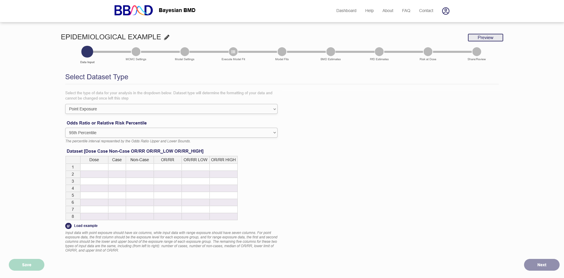
Figure 6.1. First page of a new epidemiological BMD analysis
B. Data Input
The module for epidemiological data has two options for modeling exposure. You can either model your exposure as a point value or as a range. The range exposure function uses a bootstrap method to model the uncertainty in your exposures. This method requires more computational overhead and thus takes significantly longer to execute. You can choose which exposure modeling to use in the first drop down.
To analyze an epidemiological dataset, you’ll need to input it into the system. An epidemiological dataset has either 6 or 7 columns depending on which exposure type is selected. The first column is either the point exposure or dose or if range exposure is selected there will be two columns one for the lower bound of the exposure and one for the upper bound. These columns are “Dose Low” and “Dose High”. If you’re using range exposure the Dose Low should be the lowest observed exposure in the group and Dose High should be the highest. Next, is the number of Cases then the number of Non-Cases. Next is the Odds Ratio followed by the lower and then upper bounds for the Odds Ratio. Whether you want to use the 95th or 90th percentile as the bounds for the odds ratio can be toggled using the drop-down menu. For an explanation on the Odds Ratio including how to calculate it see here.
C. MCMC Settings
On this tab (shown in Figure 6.2), you can specify some settings for the MCMC algorithms.
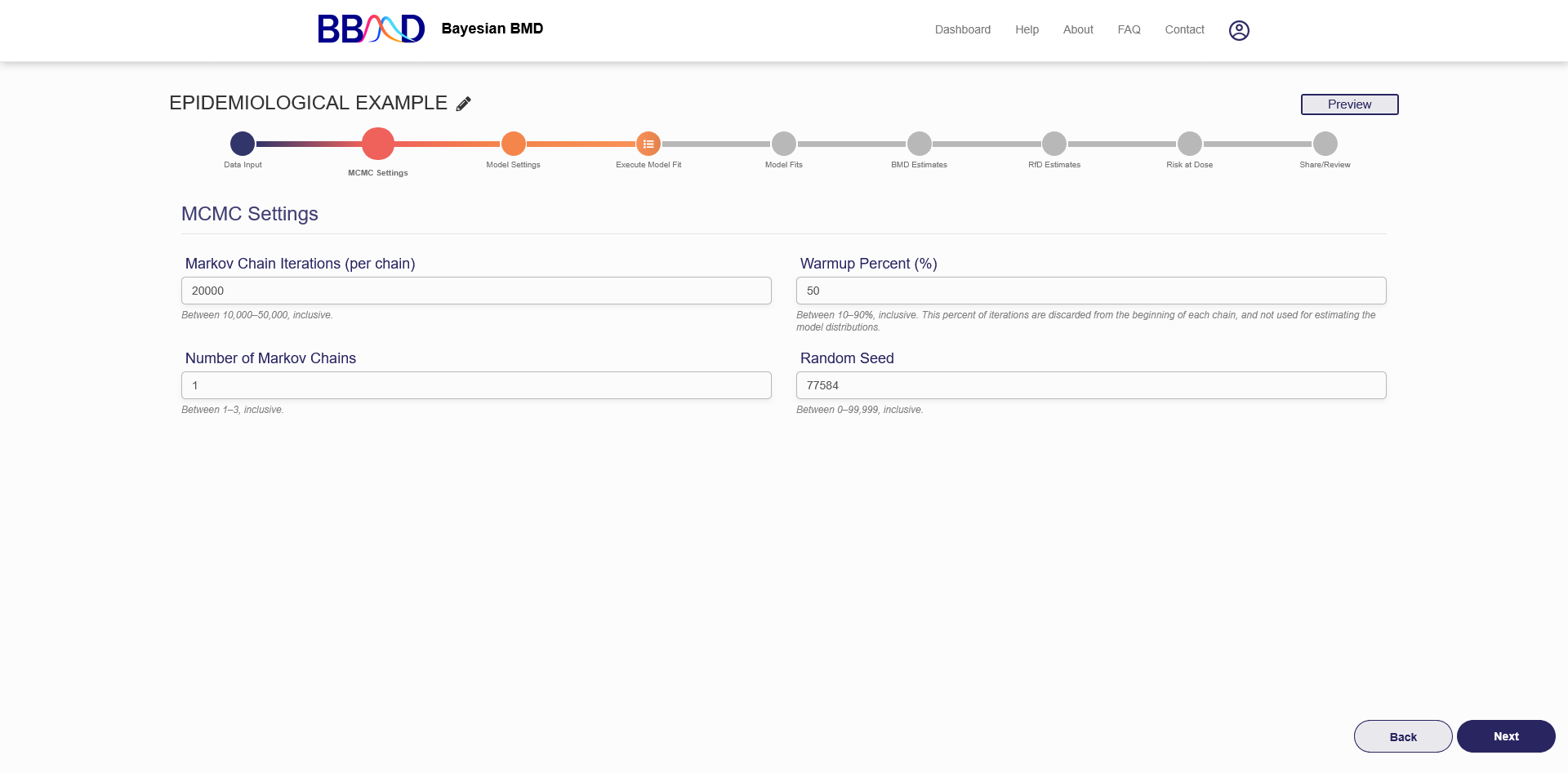
Figure 6.2. MCMC settings
There are four different values that need to be specified in this tab. First, specify the number of Markov chain iterations, between 10,000 and 50,000 (inclusive) iterations per chain. Enter your value into the “Markov Chain Iterations” text box. Next, you need to specify the warmup percentage for each Markov Chain. This is the percentage of iterations discarded from the beginning of each chain; Therefore, those iterations will not be used for estimating model distributions. Put this percentage in the “Warmup Percent (%)” text box. Third, specify the number of Markov chains used in the analysis. Enter a number 1 to 3 (inclusive) into the “Number of Markov Chains” text box. Each chain will use the number of iterations previously specified. The final value is the random seed which is used for reproducing analysis results. The random seed can be 0 to 99,999 (inclusive). Enter this value in the “Random Seed text box”.
Once these values are specified, click “Next” to save the MCMC settings and move to ‘Model Settings’. Default settings are generally acceptable. However, results in the next step will provide important information that can help you judge if the MCMC settings are appropriate. Based on our testing, the default settings are adequate for most of the commonly seen dose-response shapes, so we suggest you use the default settings for your initial run.
“Iterations” is the length of MCMC chain, i.e., the number of posterior samples in each MCMC chain. Default value is 30,000. The allowable range is any integer between 10,000 and 50,000.
“Number of chains” is the number of Markov Chains to be sampled. Default value is 1. Allowable range is 1 - 3.
“Warmup percent (%)”, the percent of sample in each Markov Chain will be discarded from the final posterior sample. Default value is 50% with an allowable range of 10% - 90%.
“Seed” is random seed number used in the MCMC algorithms. The number is randomly generated, but you can specify the number for the purpose of reproduction.
D. Model Settings
After the MCMC settings tab is the model settings tab. In this tab you choose which dose response models to fit to your dataset. The Epidemiological module has the same 8 models as the continuous module. Briefly these are:
- Exponential 2
- Exponential 3
- Exponential 4
- Exponential 5
- Hill
- Power
- Michaelis Menten
- Linear
You can choose individual models or choose “Standard Models” to add all 8 models. After choosing your models click execute to begin fitting the models.
E. Model Fit Results
On the “Model Fit Results” tab, the model fitting results obtained from the previous step are displayed. Click the name of one of the models on the left panel, then the results will be shown on the right (as shown in Figure 6.3) These results include the textual output of model parameter estimation, dynamic dose-response plot, posterior predictive p-value, model weight, correlation matrix, and graphical output of posterior sample of the model parameters (hidden by default). When click “Hide Parameters”, the parameter charts for each parameter in the model are displayed as shown in Figure 6.4.
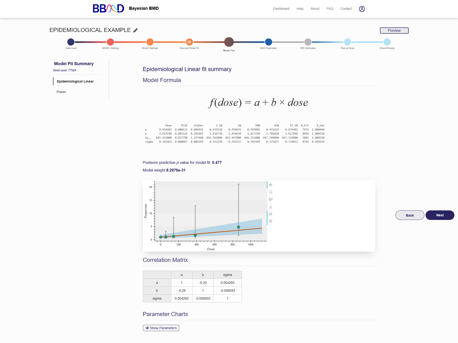
Figure 6.3. Results Shown on the “Model fit Results” Page
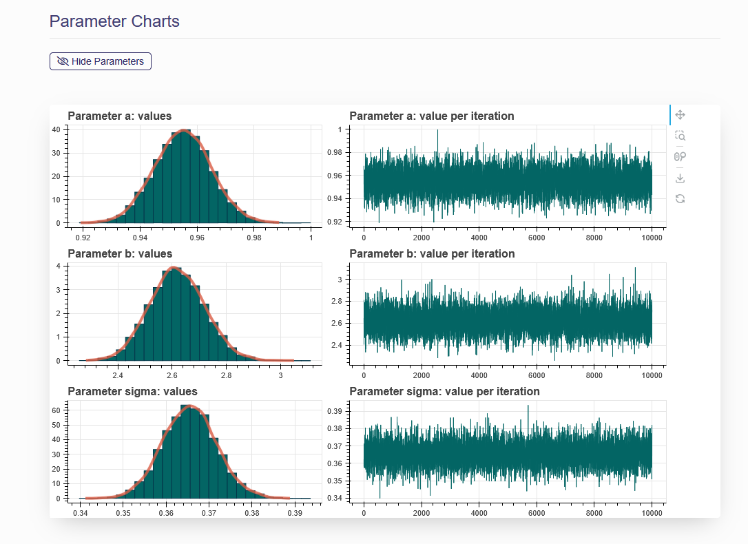
Figure 6.4. Parameter Charts
Parameter estimation results
The parameter estimation results, displayed in a table under the model formula, show the statistical summary for the estimated posterior distributions of parameters in the given dose-response model. These results are obtained directly from PyStan’s fit output, including some important statistics for model parameters and diagnostic indictors for the MCMC algorithms. The mean, standard error of the mean (MCSE), standard deviation (StdDev), various quantiles (2.5%, 25%, 50%, 75%, and 97.5%), and quantities indicating effective sample size (N_Eff) and chain convergence (Rhat) for each model parameter derived from the posterior distribution of each parameter, as well as information regarding the MCMC execution are summarized in the table. As a note, the “Rhat” can be used to judge if the MCMC chains have converged properly. If the Rhat value is larger than 1.05, you may consider increasing the length of MCMC chains to get better convergence.
Posterior Predictive P-Value
A posterior predictive p-value (PPP value) is reported below the dynamic dose-response plot. The PPP can be approximated by counting the predicted responses that satisfy the inequality out of the entire posterior sample space. This indicator can be used to judge if the fitting of this particular model is adequate. A large or small p-value means that a discrepancy in predicted data is very likely, further indicating a poor fit. Practically, if the PPP value is between 0.05 and 0.95, then the fitting is adequate. The calculation procedure of PPP value is briefly described below:
- Use each bundle of parameters in the kept posterior sample to form a dose-response model and randomly generate case numbers, 𝑦𝑟𝑒𝑝, at all dose levels in the original dataset
- Use posterior sample of model parameters to calculate a test statistic for both the original data set (𝑑, 𝑛, 𝑦) and the replicated data set (𝑑, 𝑛, 𝑦𝑟𝑒𝑝). The test statistic used in this system is log-likelihood. For parameter values from l-th iteration, we have statistic 𝑇(𝑦, 𝜃𝑙) and 𝑇(𝑦𝑟𝑒𝑝, 𝜃𝑙).
- For l = 1, …, L (the length of posterior sample), compare each pair of 𝑇(𝑦, 𝜃𝑙 ) and 𝑇(𝑦𝑟𝑒𝑝, 𝜃𝑙), and count the number of 𝑇(𝑦, 𝜃𝑙) > 𝑇(𝑦𝑟𝑒𝑝, 𝜃𝑙), say 𝑀
- The posterior predictive P-value is 𝑀/𝐿
A detailed explanation on this procedure can be found in the Chapter of “Model checking and improvement” in Bayesian Data Analysis (Gelman et al).
Posterior Model Weight
A model weight (𝑚̂𝑗) for model j is calculated for each model included in the analysis as a statistic for cross-model comparison. The model weight was introduced by (Wasserman, 2000), using the following two equations. The 𝑚̂𝑗 value of each selected model j is calculated as follows:
𝑚̂𝑗 = exp (ℓ̂𝑗 − (𝑑𝑗/2)×𝑙𝑜𝑔(𝑛))
where ℓ̂𝑗 is a loglikelihood value estimated using one set of posterior samples of model parameters of the jth model, 𝑑𝑗 is number of parameters in the jth model, and 𝑛 is the sample size in the data set.
When all models in the analysis have an equal prior weight, the posterior model weight of model j is calculated by m value estimated from model j divided by the sum of m values estimated from all models in the analysis as the following equation.
Pr(ℳ𝑗|𝐷𝑎𝑡𝑎) = 𝑚̂𝑗/∑ 𝑚̂t
This function assumes equal model priors for all models selected, so the weight mainly indicates how well the model fits the data. To make the weight more reliable, we use 1000 sets of randomly selected posterior samples of model parameters to calculate the model weights. This model weights are further applied to the model averaged BMD calculation in the F. BMD Estimation section.
Interactive Dose-Response Plot
A dynamic dose-response plot is shown below the text box. This plot includes original dose-response data and a fitted curve with its 90th percentile interval shaded in blue. When you move your mouse over the dose-response curve, the estimated median and the 5th and 95th percentiles at a particular dose level will display. When you move your mouse over a data point from your inputted dataset, the dose, N, incidence, and the response percentile will also be displayed. Other information displayed in this figure includes the PyStan version, the lower bound placed on the power parameter (if applicable), the posterior predictive p-value (PPP value) for model fit and model weight for cross-model comparison.
Correlation Matrix
The fourth item displayed is the correlation matrix for the different model parameters. The correlation matrix is to show the correlation coefficients between different model parameters and is calculated using posterior samples.
Plots for parameter posterior sample
If you click the “Show Parameters” under Parameter Charts, two plots (posterior sample trace plot and estimated probability density plot) will be displayed for each of the parameters in this dose-response model.
Basically, this is the results display tab, meaning that you can only review the results, not give the system additional inputs to modify the results.
F. BMD Estimation
On this page, you can calculate the BMD estimates of your interest. The settings for epidemiological BMD estimates are similar to those for continuous data but differ in a few key ways. For Epidemiological BMDs each BMR is expressed in terms of a relative change from the response at some background exposure level. Figure 6.5 shows the screenshot for epidemiological BMD estimation
You can change the name of the BMD Settings using the first field. This has no effect on the actual BMD calculations, but does make it easier to navigate the BMD settings page when you have multiple BMDs. Next is the “Benchmark Response Value”. The BMR is expressed in terms of relative change from the background value. There are three options to specify the “Background Exposure Level”. Each option can be selected from the drop down menu. The first “Reference Group” sets the Background Exposure Level equal to the lowest exposure group. If you’re using an exposure range this value is the halfway between the lower and upper bounds of the range. The second background exposure option is to set the background exposure to zero. Finally, the “Custom” option allows the user to set the background exposure to any value. The system also allows you to specify the prior weight for each model. These prior weights should not consider the model fits on the previous tab as this information is already included in the algorithm to calculate the posterior weights. After you specify the settings click “Execute” to calculate the BMD.

Figure 6.5. Epidemiological BMD settings
After executing the BMD will be displayed as a summary table and posterior plots of the BMD for the model average and for each model will be displayed. An example for epidemiological BMD estimation can be seen in figure 6.6 and Figure 6.7.
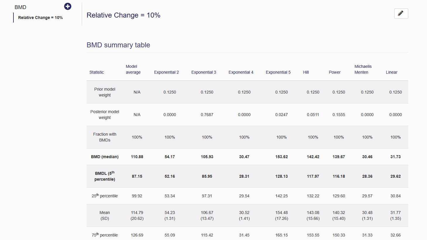


Figure 6.6. Epidemiological BMD estimation summary table
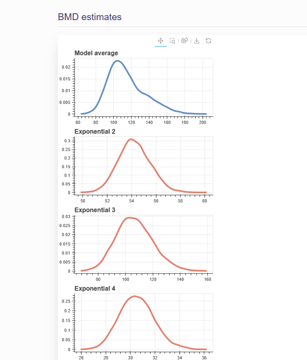
Figure 6.7. Posterior Plots of Epidemiological BMDs
