A. Introduction to BMD analysis for Genomic Data

This analysis is designed to perform BMD modeling and estimation for genomic data.

When beginning a new analysis, an automatically generated name “New Genomic BMD Analysis Month Day Year, HH:MM AM/ PM” is assigned to the analysis. You can click the pencil button next to the analysis name, as seen in Figure 4.1, to make the name more identifiable.

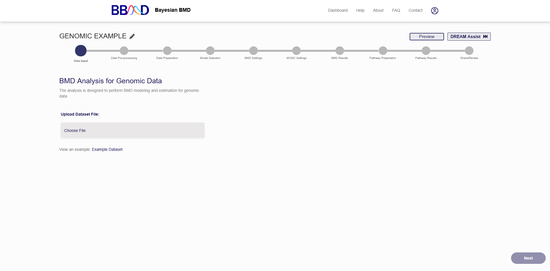
Figure 4.1. First page of a new genomic BMD analysis

B. Data Input

The first step in performing a BMD Analysis for genomic data is to input your genomic dataset. The dataset needs to be inputted as a “.csv” file and contain the proper columns/rows. The first row should be the Sample IDs, followed by the second row which should contain the dose levels. After that, each row should be labeled with the Gene name. Each column should be a different sample ID and dose level. The table below shows the first few columns and rows of an example dataset.

Example Genomic Dataset

                                                                                                        …

 The row labels “SampleID” and “Dose” must be present in the dataset, otherwise the dataset will be considered invalid.

After a dataset is successfully uploaded, a summary table, principal component plots, and a density plot will be available to view, as shown in Figure 4.2. The summary table will show the dataset file name, the number of doses, the dose levels, the number of samples, number of valid genes, and invalid genes (if any were present). An invalid gene is a gene with insufficient data, such as missing response values. If your dataset contained invalid genes, those genes were removed, and you can continue the analysis with the remaining genes.

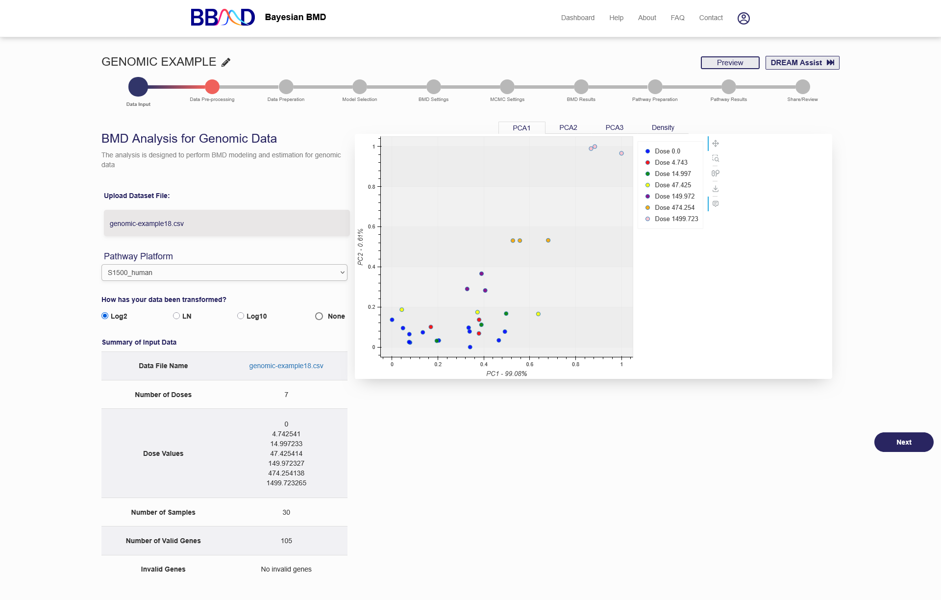
Figure 4.2. Summary results and the plots available after successfully uploading a genomic dataset

There are also four different plots available to display the relationships found within the data. The first three plots are Principal Component plots, showing PC1 vs. PC2, PC1 vs. PC3, and PC2 vs. PC3. For these plots, each dose level is given a unique color, and you can hover over the points on the plot to show their dose level and sample ID. The PCA plots are intended to demonstrate how well the genomic data clustered before performing an analysis. PCA plots can be used to identify the outlier samples that seem “far away” from others in their replicate group. The outliers may reflect some biological interactions that should not be ignored depending on your experimental system. Combining the PCA plots and the density plot to decide if data should be included in the analysis or not. The last plot is the Density plot, which gives you an idea about the signal distribution across microarray chips.  Arrays that have very different distributions in the density plot should be checked carefully. Generally, these arrays will show up as problematic and if so, should be removed before analysis.

Before you can continue onto data pre-processing, you must input the type of transform the data has already undergone. The options are log2, ln, or log10. If the data has not yet been transformed, select “None”, and a log2 transform will be applied. The transform type is necessary for the preprocessing algorithms, so it is critical that the correct option is selected.

Once have finished the data transform step and are satisfied with the summary data, you can click “Next” in the bottom right corner to continue onto the “Data Pre-processing” tab.

C. Data Pre-processing

The next step in performing a genomic BMD analysis is to use the three preprocessing algorithms to rule out genes that don’t fit the specified criteria. This step will reduce the number of genes to be used in the analysis in the BMD analysis and Pathway analysis steps. Figure 4.3 shows the “Data Pre-screening” tab before the preprocessing algorithms have executed.

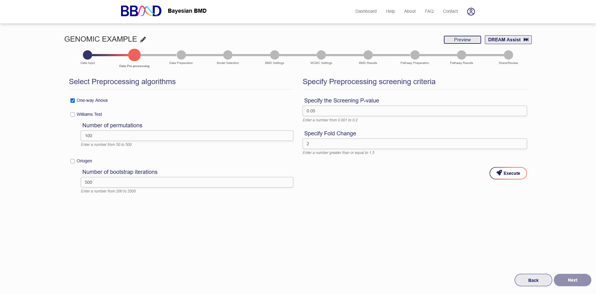
Figure 4.3. “Data Pre-processing” tab for a Genomic BMD Analysis

Performing data preprocessing takes place in two steps. The first step is to choose the preprocessing algorithms to use and specify the required settings. The second step is to specify the preprocessing screening settings.

The three algorithms used for preprocessing are “One-way Anova”, “Williams Test”, and “Oriogen”. All three of the algorithms use the same screening criteria to select genes that pass, but the screening values are calculated differently in each algorithm, so different genes may pass one algorithm but not another. If you use either “Williams Test” or “Oriogen” you must also specify an additional setting. For the “Williams Test”, you must enter the number of permutations to be used during the algorithm, and for “Oriogen” you must specify the number of bootstrap iterations to be used during the algorithm. Using a higher number of permutations or bootstrap iterations may allow the algorithms to become more precise but with the cost of taking longer to execute.

The screening criteria that you need to specify is the screening P-value and the fold change. For a gene to pass prescreening, the P-value must be below the value entered in the corresponding text box. The gene’s fold change must be above the value entered into that text box.

Once you are satisfied with the selected algorithms, algorithm settings, and prescreening criteria, press “Execute” in the lower right corner. The prescreening algorithms can take a long time to execute, so an email will be sent to your inbox when the prescreening is complete so you can return to the analysis to view the results and move onto BMD and Pathway analyses.

When the preprocessing algorithms have finished executing, a summary of the results, and two volcano plots will be displayed, shown in Figure 4.4. The summary of results will show the number of genes that passed each prescreening algorithm. The volcano plots will show the max fold change vs. the adjusted p-value and unadjusted p-value for each gene that passed the prescreening. These genes will be marked by different colors on the volcano plot, depending on the prescreening algorithm used. You can also hover over the markings on the volcano plot to see the specific gene name so that you can remove or add these genes from your BMD datasets on the next tab.

Note: If the unadjusted or adjusted p-value of a gene is too close to 0, the system may not include these on the plot because Log(p-value) will be undefined.

If you are not satisfied with the prescreening results, you can change the settings and re-execute the prescreening algorithms. Like before, an email will be sent to your inbox when the prescreening has completed.

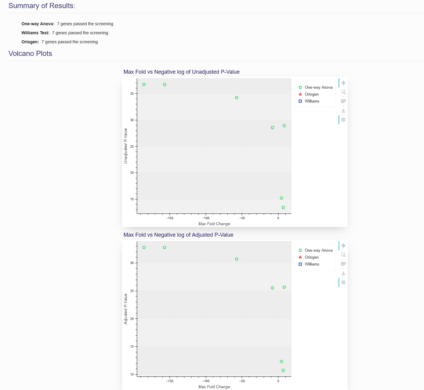
Figure 4.4. Preprocessing Summary and Volcano plots

Criteria including fold changes, P-values, adjusted P-values are applied to filter gene expression data.

Fold Change

𝑓 = {𝑎𝑏𝑠 max (− 1/𝑏𝑎𝑠𝑒^(𝑥_𝑖−𝑥₀)); 𝑖𝑓 𝑏𝑎𝑠𝑒(𝑥_𝑖−𝑥₀) < 1
𝑎𝑏𝑠 max (𝑏𝑎𝑠𝑒^(𝑥_𝑖−𝑥₀)); 𝑖𝑓 𝑏𝑎𝑠𝑒(𝑥_𝑖−𝑥₀) ≥ 1

where 𝑥_𝑖 is the response at i-th dose level, 𝑥₀ is the response at control level, and base is the log base of data log transformation

P-value and Adjusted P-value

P-values are calculated by one way ANOVA and trend test (Williams test and Oriogen). With the P-values, adjusted P-values are calculated by Benjamini-Hochberg methods.

One Way Anova

One way ANOVA is a well-known test to determine whether there are any statistical differences between the means of the experiment group and the control group. The ANOVA produces an F-statistic, the ratio of the variance calculated among the means to the variance within the samples. A higher F-ratio implies that the samples were drawn from populations with different mean values. The F-ratio gives a P-value to determine whether significant differences exist in the experiment and control groups.

Williams Test and Oriogen

We adapt William’s trend test (Williams 1971, 1972) and Oriogen (Peddada et al. 2005) to identify genes having a monotonical trend with respect to doses. That is, the maximum likelihood estimate (MLE) of mean response at i-th level is estimated by equation (1) and the test statistic (𝑇) is calculated by equation (2). Permutation and bootstrap methods are applied to calculate the probability (P-value) that 𝑇𝑖 (i-th permutation or bootstrap) is larger than 𝑇.
𝜇_𝑖̂ ={𝑚𝑎𝑥_{1≤𝑢≤𝑖}𝑚𝑖𝑛_{1≤𝑣≤𝐾}∑ 𝑛_𝑗𝑋̅_𝑗/∑ 𝑛_𝑗; 𝑖𝑓 𝑖𝑛𝑐𝑟𝑒𝑎𝑠𝑖𝑛𝑔
𝑚𝑖𝑛_{1≤𝑢≤𝑖}𝑚𝑎𝑥_{1≤𝑣≤𝐾} ∑ 𝑛_𝑗𝑋̅_𝑗/∑ 𝑛_𝑗; 𝑖𝑓 𝑑𝑒𝑐𝑟𝑒𝑎𝑠𝑖𝑛𝑔
where 𝜇_𝑖̂ is the MLE of 𝜇_𝑖, 𝐾 is dose level, 𝑖 is the index of treatments group (𝑖 = 1, … , 𝐾), 𝑛_𝑗 is
the number of samples at j-th level, and 𝑋̅_𝑗 is the mean response at j-th level.
𝑇 = 𝑎𝑏𝑠 max ( (𝜇_𝑖̂ −𝑋_0̅̅̅̅)/(𝑠√1/𝑛_𝑖+ 1/𝑛₀)
where 𝑋_0̅̅̅ is the mean response at the control level, 𝑠 is an unbiased estimate of within group
standard deviation, 𝑛𝑖 is the number of samples at i-th level, and 𝑛₀ is the number of samples at
control level.

D. Data Preparation

After genes have been selected out with preprocessing, you have another opportunity to remove genes from your analysis in the data preparation step. This tab, shown in Figure 4.5, allows you to add and remove specific genes, and create multiple datasets for the BMD and Pathway analyses. 

To create a dataset, follow the three steps below:

1. Give the dataset an identifiable name in the “Dataset Name” text box.
2. Choose the preprocessing algorithm which you will select genes from for the dataset.
3. Add the desired genes to the dataset using the checkbox in the gene’s row. The sliders on the right-hand side of the page can be used to add all genes that fit those three parameters. Even after adjusting the sliders, you can individually add or remove genes using the check box.
4. When you are satisfied with the dataset, click the green “Create” button on the bottom left side of the page.

You should see the dataset name appear on the left column of the page. If you want to edit this dataset, click on the name, and then change any of the settings previously chosen. After you are finished editing, save your changes by clicking the green “Update” button in the bottom left corner. To add an additional analysis, click the plus icon next to “Datasets” in the left column, then follow steps (1) – (4) again. You may include up to three datasets per genomic analysis. If you need to use more datasets, you can begin a new genomic analysis. If you want to delete a dataset, click the three dots icon next to the dataset name, then click “Delete”. This will remove that dataset from your list to be analyzed. If you had three datasets and then delete one, you can add another.

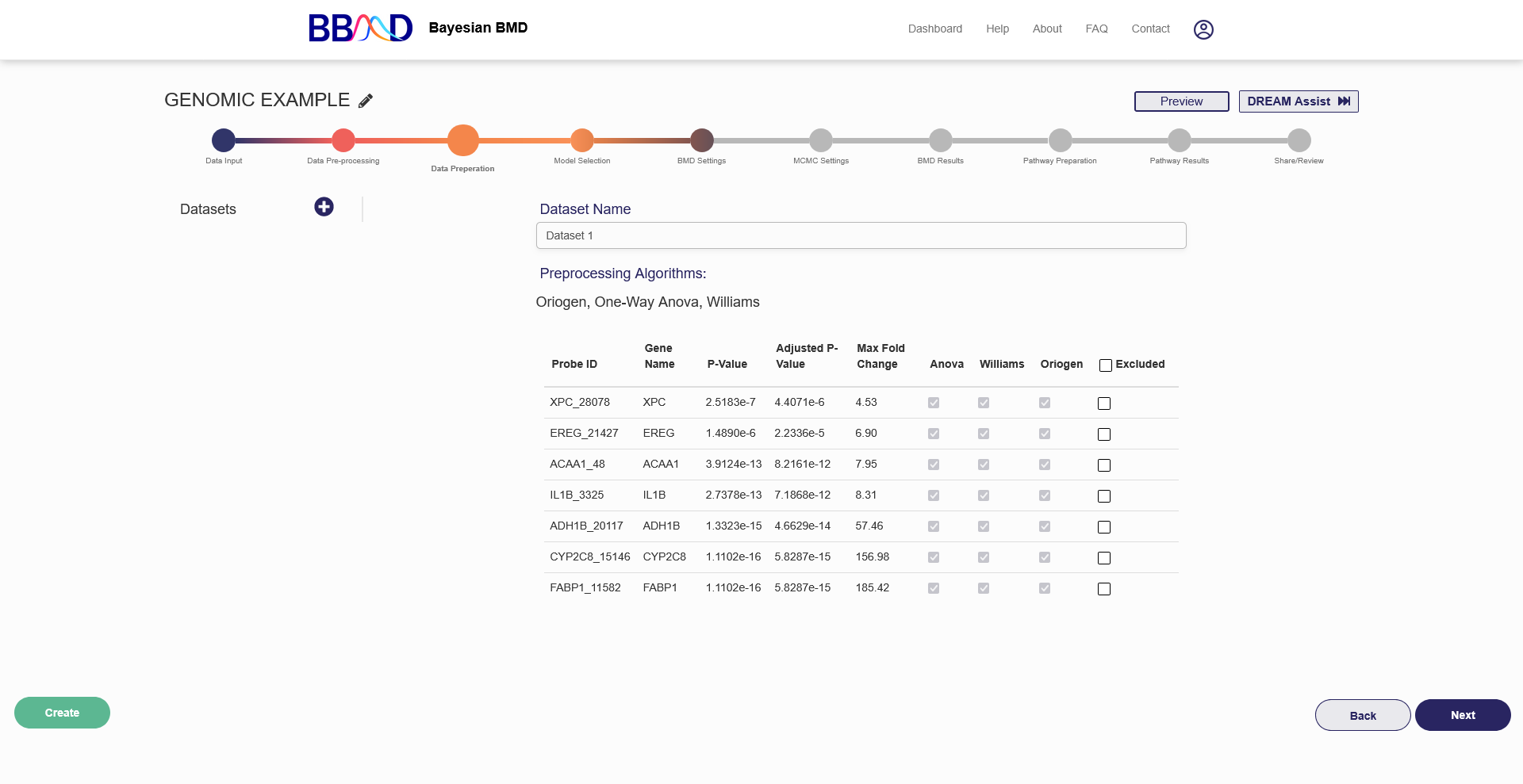
Figure 4.5. “Dataset Preparation” tab for genomic BMD analysis

E. Model Selection

Before specifying BMD settings, you must select the models to be used in the model fitting part of the analysis. 

The available dose-response models are:

1) Linear Model:
𝑓(𝑑𝑜𝑠𝑒) = 𝑎 + 𝑏 × 𝑑𝑜𝑠𝑒, 𝑎 > 0

2) Power Model:
𝑓(𝑑𝑜𝑠𝑒) = 𝑎 + 𝑏 × 𝑑𝑜𝑠𝑒^𝑔
𝑎 > 0, 𝑔 ≥ 𝑟𝑒𝑠𝑡𝑟𝑖𝑐𝑡𝑖𝑜𝑛

3) Hill Model:
𝑓(𝑑𝑜𝑠𝑒) = 𝑎 + 𝑏 × 𝑑𝑜𝑠𝑒^𝑔/𝑐^𝑔 + 𝑑𝑜𝑠𝑒^𝑔
𝑎 > 0, 𝑐 > 0, 𝑔 ≥ 𝑟𝑒𝑠𝑡𝑟𝑖𝑐𝑡𝑖𝑜𝑛

4) Exponential 2 Model:
𝑓(𝑑𝑜𝑠𝑒) = 𝑎 × 𝑒^{𝑏×𝑑𝑜𝑠𝑒} , 𝑎 > 0

5) Exponential 3 Model:
(𝑑𝑜𝑠𝑒) = 𝑎 × 𝑒^{𝑏×𝑑𝑜𝑠𝑒^𝑔}
𝑎 > 0, 𝑔 ≥ 𝑟𝑒𝑠𝑡𝑟𝑖𝑐𝑡𝑖𝑜𝑛

6) Exponential 4 Model:
𝑓(𝑑𝑜𝑠𝑒) = 𝑎 × (𝑐 − (𝑐 − 1) × 𝑒^{−𝑏×𝑑𝑜𝑠𝑒} )
𝑎 > 0, 𝑏 > 0, 𝑐 > 0

7) Exponential 5 Model:
𝑓(𝑑𝑜𝑠𝑒) = 𝑎 × (𝑐 − (𝑐 − 1) × 𝑒^{−(𝑏×𝑑𝑜𝑠𝑒)^𝑔})
𝑎 > 0, 𝑏 > 0, 𝑐 > 0, 𝑔 ≥ 𝑟𝑒𝑠𝑡𝑟𝑖𝑐𝑡𝑖𝑜𝑛

To include a model in the analysis, click the checkbox on the right side of the model’s row in the table displayed in the “Model Selection” tab (shown in Figure 4.6). When you check the box, the model is automatically added and saved to your analysis. Once you have added all the models you wish to include, press “Next” in the bottom right corner to begin specifying BMD settings.

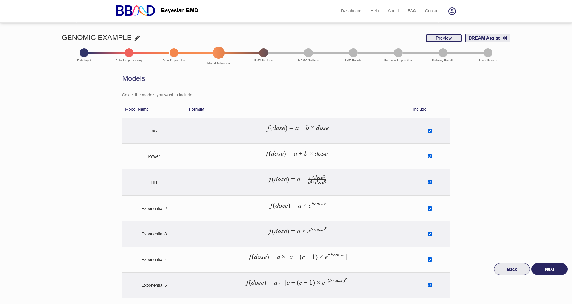
Figure 4.6. “Model Selection” tab for genomic BMD analysis

F. BMD Settings

The next step in completing a genomic BMD analysis is to specify the BMD settings (the “BMD Settings” tab is shown in Figure 4.7). Two types of BMRs are available for genomic data: SD Change and Relative Change.

To create a BMD estimate to be analyzed, complete the following four steps:

1. Choose a name for the estimate. The default name for SD change is “BMD = BMR Value SD”. The default name for relative change is “BMD = BMR Value %”. If you would like to use a more identifiable name, enter this into the “Name” text box.
2. Select a BMR Type from the corresponding drop-down menu.
3. Specify the BMR value and enter this into the “BMR Value” text box.
4. Click “Save” at the bottom of the page to save these settings.

When the settings are successfully saved you should see the BMD settings name appear on the left column of the page. To edit these settings, click the name, then follow the previous steps to change any values. Once you have made the desired changes click the green “Update” button on the bottom of the page. If you want to instead cancel these changes, click the “Cancel” button on the bottom of the page. If you would like to add a new BMD setting for this analysis, click the plus icon next to “BMD” on the left side of the page. Three BMD settings are allowed for each genomic analysis. If you would like to delete this settings definition, click the setting’s name on the left side, and then click the red “Delete” button on the bottom of the page.

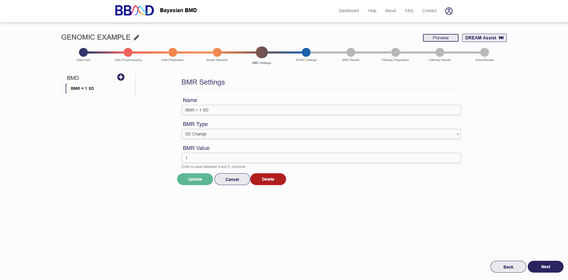
Figure 4.7. “BMD Settings” tab for genomic BMD analysis

Two options for defining the BMR values are provided based on the central tendency: a) relative change and b) standard deviation, which are descried below. In BBMD, several BMRs can be defined.

𝑓(𝐵𝑀𝐷) ± 𝑓(0) = 𝑟𝑒𝑙𝑎𝑡𝑖𝑣𝑒 𝑐ℎ𝑎𝑛𝑔𝑒 × 𝑓(0),
𝑓(𝐵𝑀𝐷) ± 𝑓(0) = 𝑘 ×standard deviation,
where 𝑓(0) is the estimated response at zero dose, 𝑓(𝐵𝑀𝐷) is the response at BMD, relative change (e.g., 10%) and 𝑘 (e.g., 1) are values defined by user, and standard deviation is estimated by models given observations. As a note, for every model, every posterior sample has an estimate for 𝑓(0), standard deviation and therefore a BMD estimated value.

G. MCMC Settings

The final step before executing the BMD analysis is to specify the MCMC settings, the “MCMC Settings” tab is shown in Figure 4.8. 

There are four different values that need to be specified in this tab. The first value is the number of Markov chain iterations, which can be 10,000 to 50,000 (inclusive) iterations per chain. Enter your value into the “Markov Chain Iterations” text box. Next, you need to specify the warmup percentage for each Markov Chain. This is the percentage of iterations discarded from the beginning of each chain; Therefore, those iterations will not be used for estimating model distributions. Put this percentage in the Warmup Percent (%) text box. The third value that needs to be specified is the number of Markov chains used in the analysis. Enter a number 1 to 3 (inclusive) into the “Number of Markov Chains” text box. Each chain will use the number of iterations previously specified. The final value is the random seed which is used for reproducing analysis results. The random seed can be 0 to 99,999 (inclusive). Enter this value in the “Random Seed text box”.

Once these values are specified, click “Save” to save the MCMC settings. If you are ready to execute the analysis, press “Execute” on the right side of the page. This will begin the BMD analysis execution. Once the execution has completed you will receive an email notification that your analysis is ready to be accessed. You will also receive a link which will send you back to the analysis to view the BMD results.

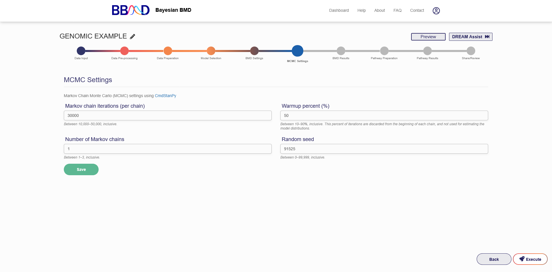
Figure 4.8. “MCMC Settings” tab for genomic BMD analysis

H. BMD Results

Once the BMD analysis has completed, the results will be displayed in the table on the “BMD Results” tab, shown in Figure 4.9. The names of the different datasets used will be shown on the left side of the page. Click the name of the dataset to view those specific results. 

For each gene, the table displays the Model name, PPP value, model weight, and then the BMD, BMDU, and BMDL for each specified BMR. The BMR name will be displayed above the BMD value, and will be the name given when the BMR settings were created.

When you are finished reviewing the results, click “Next” in the bottom right corner to advance to the platform selection tab.

You can also skip the Pathway analysis and go to the “Share/Review” tab instead by clicking the name in the tab bar. This will allow you to export BMD results to an Excel spreadsheet immediately.

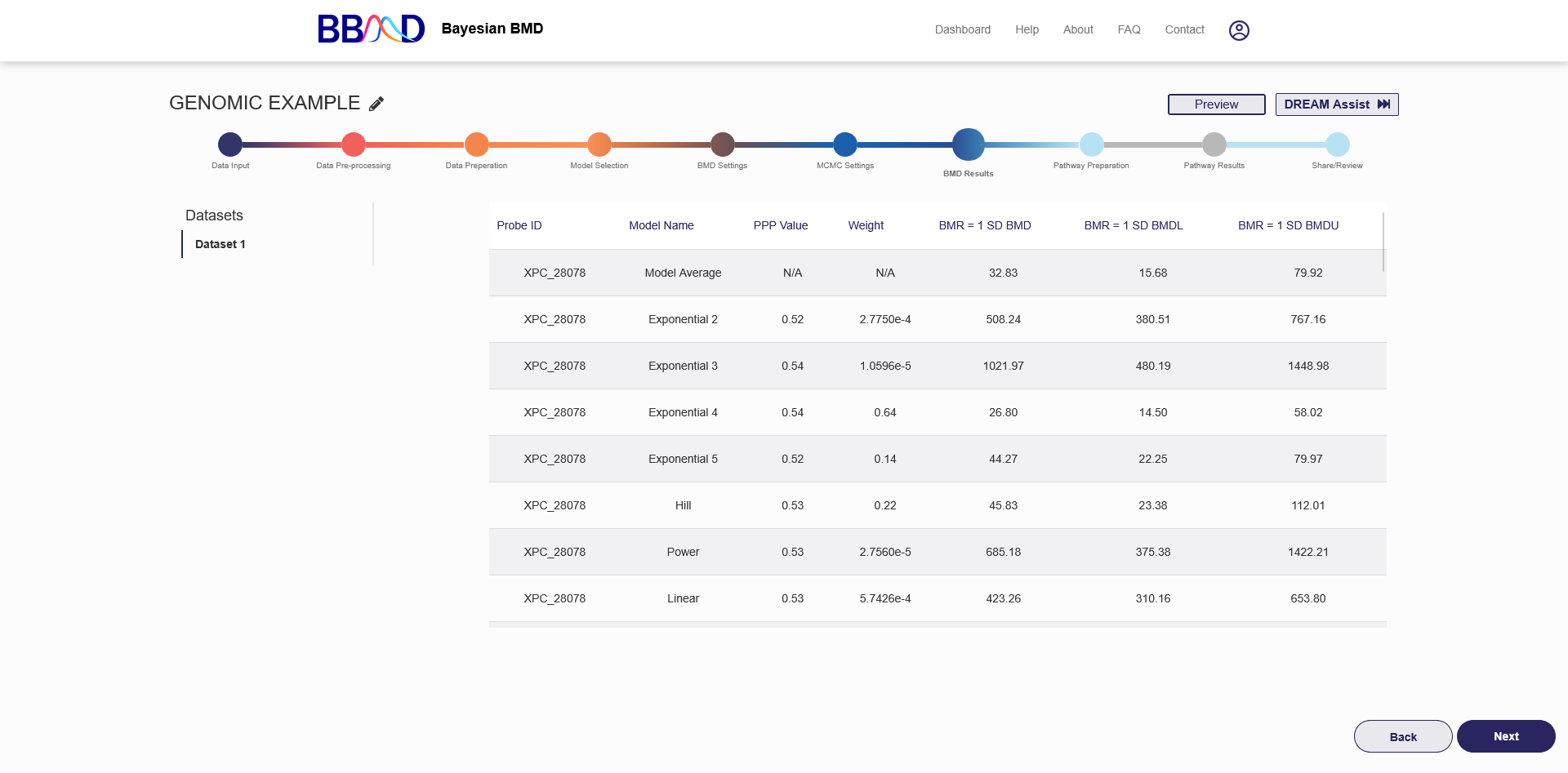
Figure 4.9. BMD Results after executing genomic analysis

I. Pathway Preparation

In this step, you must prepare for pathway BMD execution. You can use this tab to filter and select genes for pathway BMD execution based on the BMD/BMDL ratio. When you have chosen a platform, press “Execute” below the drop-down menu. Once the execution has completed, you will be able to advance to the next tab. Click “Next” in the bottom right corner to view the pathway results.

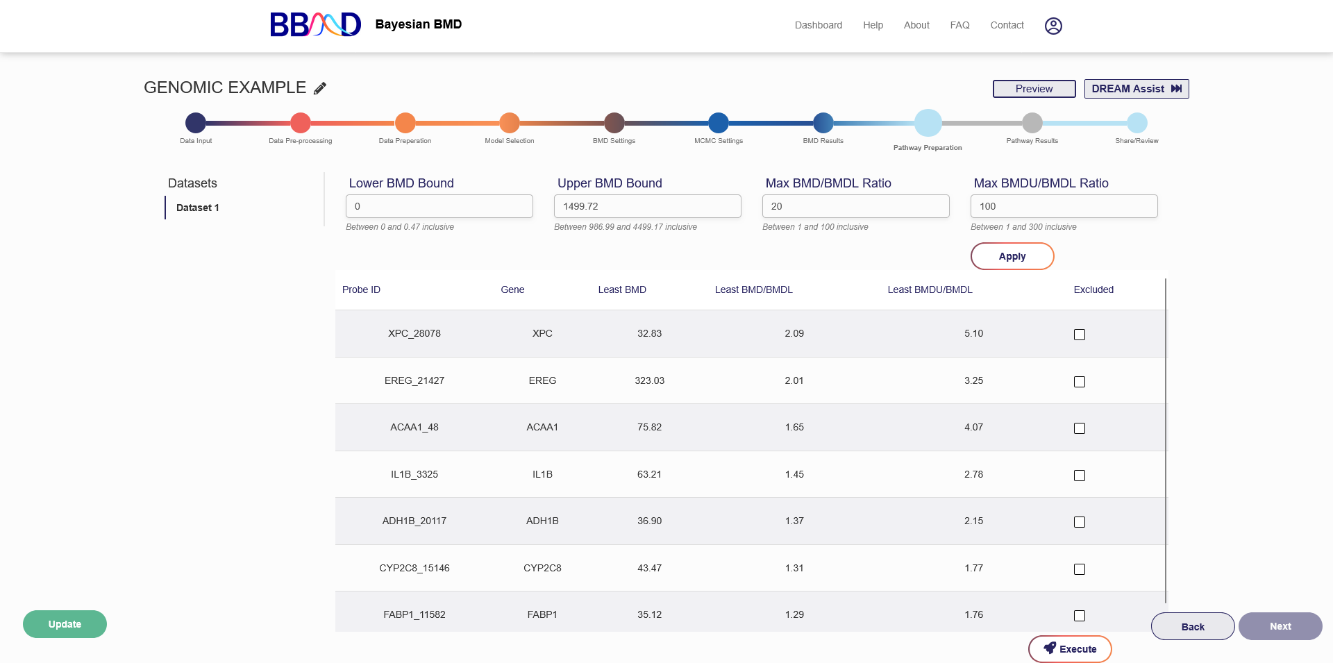
Figure 4.10. Pathway Preparation Screen

J. Pathway Analysis Results

The “Pathway Results” tab, shown in Figure 4.11, displays the results for the four different pathway types after completing a pathway analysis.

On the left side of the page, you can select the data set which you would like to view pathway results for. To switch datasets, click on the dataset name. The first section of this page is the pathway type selection. Click the pathway name to switch pathway types. The second section displays the platform summary. Summary information includes: the total number of pathways or total number of genes, number of unique genes, and then the Pathway BMD percentiles. The BMD definitions used for this analysis are the same BMDs that were used for the genomic BMD analysis. 

Below the summary section the detailed Pathway BMD results are displayed in a large table. The columns for each table are slightly different, but each table always has a “Gene ID” column or “Pathway” column. If the text appears blue and underlined in the first column, there is a link to another resource to further analyze that pathway. Similarly, the last columns of the table are always the BMD results columns for each pathway or gene ID. If the text in the results cell is blue and underlined, clicking on it will bring up a plot showing this gene’s dose level with whiskers showing the BMDL and BMDU values. If any other text is blue and underlined in the table, hover over those cells because this row corresponds to multiple Probe IDs and Gene IDs.

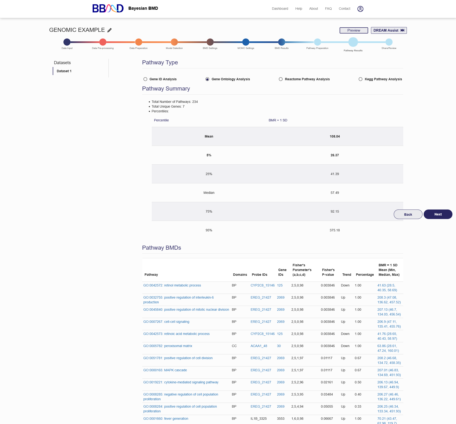
Figure 4.11. Pathway Analysis Results for “Gene Ontology Analysis”

In the pathway analyses, platforms from Gene Expression Omnibus (GEO) are provided and users need to select one that associated with the uploaded genomic data. Four kinds of pathway analyses are provided to classify the BMA BMD analyses into significant pathways based on their NCBI Entrez Gene identifiers: a) Gene ID Analysis; b) GO Analysis (Mi et al. 2019); c) REACTOME (Fabregat et al. 2018) Pathway Analysis; and d) KEGG (Kanehisa and Goto 2000)pathway analysis. Each pathway analysis, the genes were matched to their associated categories, and the minimum, maximum, average, and median BMD were calculated for each category. For each analysis, a pathway summary table and a detailed pathway BMD table are displayed. 

As for the four pathway methods, Gene ID Analysis simply translates the probe set identifiers to NCBI’s Entrez Gene identifiers. GO Analysis utilizes ‘go-basis.obo’ and a python package GOATOOLS (Klopfenstein et al. 2018) to group the Entrez Gene identifiers into three sub-ontologies: biological process, cellular component, and molecular function. The ‘reactomepy’ python module is used to access the REACTOME database, and API request is used to access the KEGG database. 

For all the analyses, probe sets that measured more than one gene were removed from analyses. When different probe sets are associated with the same Entrez Gene identifiers, mean values of BMD are taken to represent the BMD value of the Entrez Gene identifiers. In order to determine whether the pathway is significant, P-values and percentages are calculated for each category. P-values are calculated based on Fisher’s exact two-tailed test by comparing the numbers of genes with BMD estimates with the numbers of genes without BMD estimates. For each category, percentage is defined as the ratio of the number of genes with BMD estimates that are on this category to the total number of genes that are related to this category. The trend (‘Up’, ‘Down’ or ‘Conflict’) for each pathway is also provided. "Up" indicates > 60% genes in the category show up-regulation, "Down" indicates >60% show down-regulation and "Conflict" indicates neither "Up" or "Down" criteria were met.

K. Share/Review

The final tab for a genomic BMD analysis is the “Share/Review” page, shown in Figure 4.12. From this tab you can share this analysis with others and export the calculated results. 

If you would like to share your analysis with others, you can change the settings from “Private” to “Send Back”, “Share”, or “Dream Assist”. The “Share” setting allows you to send the created URL to others for them to access and review (but not edit) the analysis. The “Send Back” setting allows you to Return to the member that requested the DREAM Assist once reviewed. Lastly, the “DREAM Assist” setting will share this analysis with the DREAM Tech team, who can assist with the analysis. The  “DREAM Assist” settings are coming soon.

You can also export the results of the analysis into Excel format. Before exporting results, you can customize the parts of the analysis included on the reports. By clicking “show more” on the right side of the page, the customization options will appear. From here you can select which datasets to include in the exported results. If you wish to change the report settings in the future, you can return to this analysis and export a new report. Exporting the results will send a link to your account’s email where you can download the reports. 

At any time during the updating or reviewing stage, if you want to change to another existing analysis, you can click the “Dashboard” button on the top right corner to switch to the summary page for the existing analyses and access another analysis.

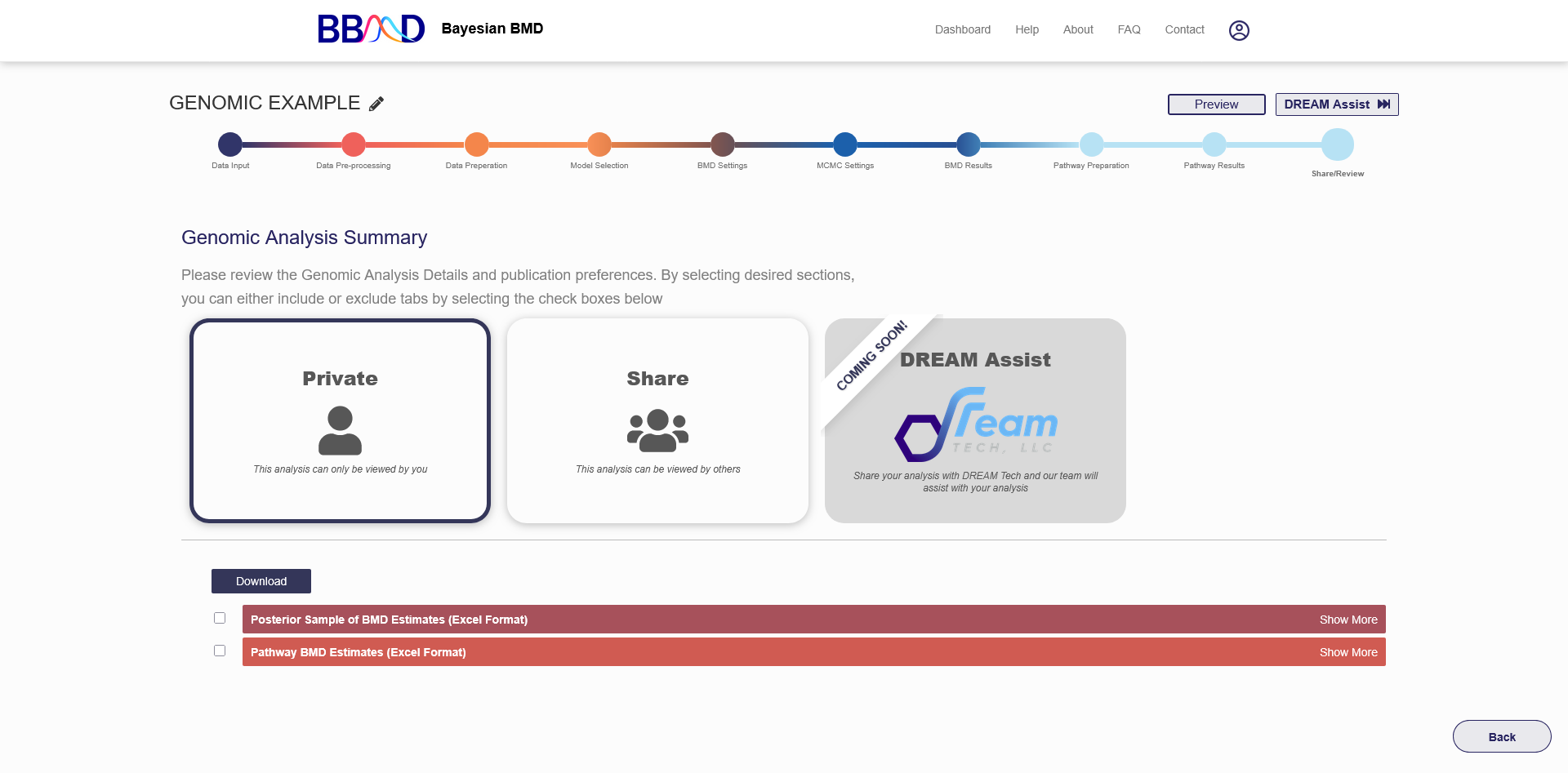
Figure 4.12. “Share/Review” tab for a genomic BMD analysis