A. Introduction to Multisite Tumor BMD Analysis

This module is designed to perform BMD modeling and estimation for multiple tumor sites. Be aware this module makes the common assumption that each tumor site is conditionally independent (conditional on the dose level). 

When beginning a new analysis, an automatically generated name “New MS Combo Run Month Day Year, HH:MM AM/PM” is assigned to the analysis. You can click the pencil button next to the analysis name, as seen in Figure 7.1, to make the name more identifiable.

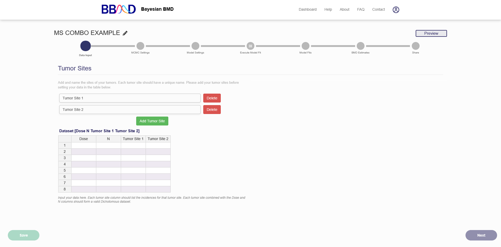
Figure 7.1. First page of a new MS Combo BMD analysis

B. Data Input

Setting your tumor sites

The Multisite Tumor module allows you to analyze up to five tumor sites. The default setup has two tumor sites but additional tumor sites can be added using the “Add Tumor Site” button. If you add too many sites you can delete some using the delete buttons to the right of the name fields. Tumor sites can be renamed by editing the text in the text box. This doesn’t affect the BMD calculations but does serve to help organize and track each tumor site. The names must be unique.

How to input data into the system

To analyze a dataset, you’ll need to input it into the system. A Multisite Tumor dataset is made up of several dichotomous datasets combined together. Like a dichotomous dataset the first two columns are the dose and the sample size (N). Then each Tumor site should have the incidence for that tumors at that particular site listed in its column. So if you have a control group with 50 animals and three with a tumor at Tumor Site 1 and four with a tumor at Tumor Site 2 the first row of your dataset would be 0   50   3   4. This is true regardless of whether an animal has tumors at sites 1 and 2 or not.

C. MCMC Settings

On this tab (shown in Figure 7.2), you can specify some settings for the MCMC algorithms.

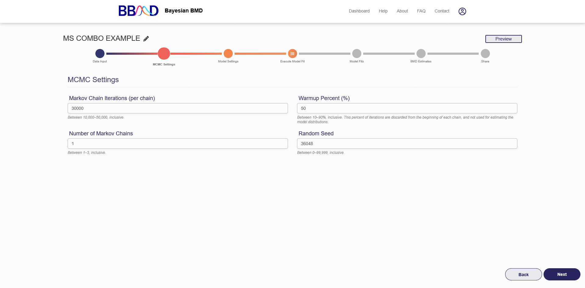
Figure 7.2. MCMC settings

How to make and change settings

There are four different values that need to be specified in this tab. First, specify the number of Markov chain iterations, between 10,000 and 50,000 (inclusive) iterations per chain. Enter your value into the “Markov Chain Iterations” text box. Next, you need to specify the warmup percentage for each Markov Chain. This is the percentage of iterations discarded from the beginning of each chain; Therefore, those iterations will not be used for estimating model distributions. Put this percentage in the “Warmup Percent (%)” text box. Third, specify the number of Markov chains used in the analysis. Enter a number 1 to 3 (inclusive) into the “Number of Markov Chains” text box. Each chain will use the number of iterations previously specified. The final value is the random seed which is used for reproducing analysis results. The random seed can be 0 to 99,999 (inclusive). Enter this value in the “Random Seed text box”.

Once these values are specified, click “Next” to save the MCMC settings and move to ‘Model Settings’. Default settings are generally acceptable. However, results in the next step will provide important information that can help you judge if the MCMC settings are appropriate. Based on our testing, the default settings are adequate for most of the commonly seen dose-response shapes, so we suggest you use the default settings for your initial run.

How MCMC settings may impact the result

“Iterations” is the length of MCMC chain, i.e., the number of posterior samples in each MCMC chain. Default value is 30,000. The allowable range is any integer between 10,000 and 50,000.

“Number of chains” is the number of Markov Chains to be sampled. Default value is 1. Allowable range is 1 - 3.

“Warmup percent (%)”, the percent of sample in each Markov Chain will be discarded from the final posterior sample. Default value is 50% with an allowable range of 10% - 90%.

“Seed” is random seed number used in the MCMC algorithms. The number is randomly generated, but you can specify the number for the purpose of reproduction.

D. Model Settings

After the MCMC settings tab is the model settings tab. In this tab (Figure 7.3) you choose which dose response models to fit to your dataset. Due to the assumptions made about conditional independence only two of our 8 dichotomous models are suitable for the Multisite Tumor module. They are the Quantal Linear and Multistage models. Each model can be included by checking the associated box or excluded by unchecking the box. You can choose whether to use our objective priors or our empirical informative priors from the prior settings menu. At least one model must be selected before clicking “Execute”.

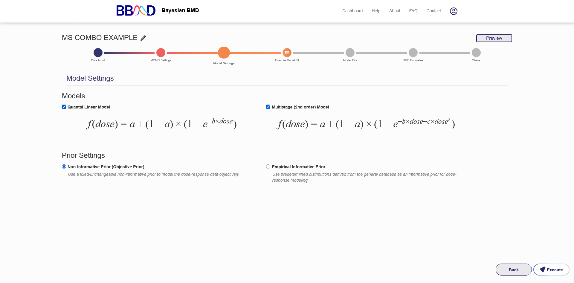
Figure 7.3. MS Tumor Model Settings

E. Model Fit Results

On the “Model Fit Results” tab, the model fitting results obtained from the previous step are displayed. Click the name of one of the models on the left panel, then the results will be shown on the right (as shown in Figure 7.4) These results include the textual output of model parameter estimation, the combined model formula, model weight, and dynamic dose response plot for each tumor site model (Figure 7.5).

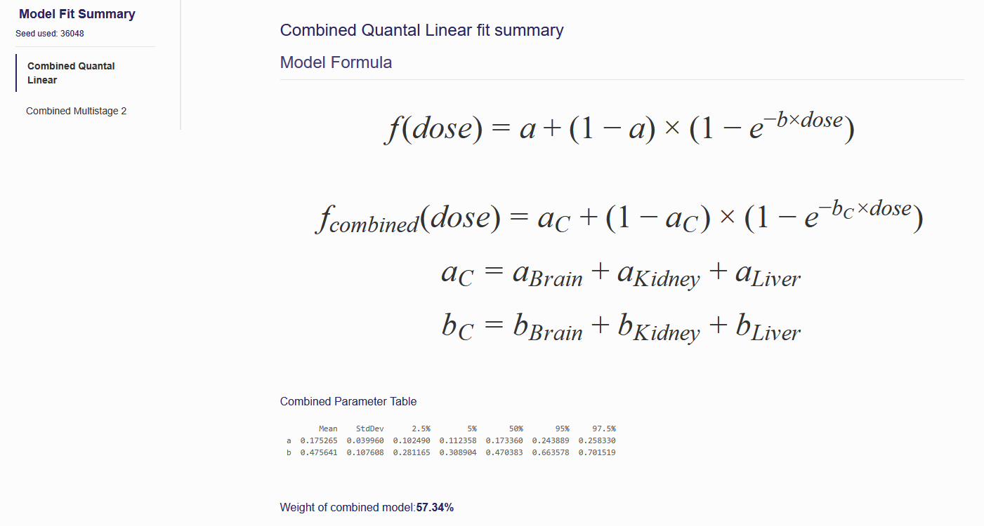
Figure 7.4. Results Shown on the “Model fit Results” Page

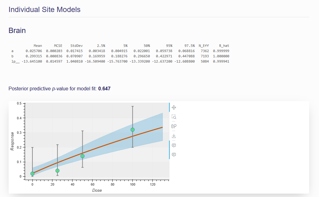
Figure 7.5. Example of an individual tumor site model

Parameter estimation results

The parameter estimation results, displayed in a table under the model formula, show the statistical summary for the estimated posterior distributions of parameters in the given dose-response model. The mean, standard error of the mean (MCSE), standard deviation (StdDev), and various quantiles (2.5%, 25%, 50%, 75%, and 97.5%) for each model parameter derived from the posterior distribution of each parameter are summarized in the table. 

Posterior Model Weight

A model weight () for model j is calculated for each model included in the analysis as a statistic for cross-model comparison. The model weight was introduced by (Wasserman, 2000), using the following two equations. The  value of each selected model j is calculated as follows:

where  is a loglikelihood value estimated using one set of posterior samples of model parameters of the j-th model,  is number of parameters in the j-th model, and  is the sample size in the data set.

When all models in the analysis have an equal prior weight, the posterior model weight of model j is calculated by m value estimated from model j divided by the sum of m values estimated from all models in the analysis as the following equation.

This function assumes equal model priors for all models selected, so the weight mainly indicates how well the model fits the data. To make the weight more reliable, we use 1000 sets of randomly selected posterior samples of model parameters to calculate the model weights. This model weights are further applied to the model averaged BMD calculation in the F. BMD Estimation section.

Individual Tumor Site Models

The models for each individual tumor site are shown under the combined model. Each individual model has its own textual output table, interactive dose response plot, and posterior predictive p value displayed.

F. BMD Estimation

On this page, you can calculate the BMD estimates of your interest. The Multisite Tumor BMD calculations are similar to those for dichotomous data.

You can change the name of the BMD Settings using the first field. This has no effect on the actual BMD calculations but does make it easier to navigate the BMD settings page when you have multiple BMDs. Next is the Benchmark Response Value. The BMR is calculated using both the added and extra risk definitions.

Figure 7.6. MS Tumor BMD settings

After executing the BMD will be displayed as a summary table and posterior plots of the BMD for the model average and for each model will be displayed.