A. General Introduction on BMD Analysis

After you selected “BMD Analysis for Single Dataset” and specified the data type in Figure 1.8, the web page will change to the one as shown in Figure 2.1. An automatically generated name, “New Continuous/Dichotomous/Categorical Run Month Day Year, HH:MM AM/PM”, is assigned to the newly started analysis. You can click the pencil button next to the analysis name, as shown in the Figure 2.1, to make the name more identifiable. Without inputting any data, you will not be able to continue to advance through the tabs. The first step in an analysis is to input dose-response data. For continuous and dichotomous data, whether the dataset is “summary” or “individual” needs to be specified. After each step is finished, the “Next” button and the tab in the progress bar will light up.

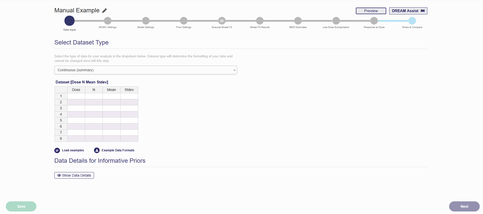
Figure 2.1. The Start Page of a New Analysis

As a note, if you would like to preview the results or view the results from the perspective of someone the analysis was shared with, click the blue button labeled “Preview” in the upper right corner (Figure 2.1). This will take you out of the updating mode. To resume updating the analysis, click the blue button labeled “Actions” in the upper right corner, and then in the drop-down list that appears, click “Update” (Figure 2.2). You can select “Edit a Copy” to create an editable copy of the analysis.

Figure 2.2. Preview mode

B. Data Input and Pre-analysis

The first tab, which is presented after confirming the selected data type, is the dataset input tab. Select the specific type of data from the dropdown menu, and then put the data into the text box. For continuous and dichotomous datatypes there will be two options in the dropdown menu: Either summary or individual data. If you are doing an analysis with categorical data, there is only one option. Each type of data requires different columns. The following section will explain the types of columns needed for each data type.

Dichotomous summary

If you choose “Dichotomous summary” for dichotomous data, three columns are required for input (from left to right): dose level, total number of subjects and number of subjects affected. The values can be pasted or manually typed, using spaces between values. Different dose groups should be entered in different rows. Below is an example dichotomous summary dataset:

Dose	N (Number of Subjects)	Incidence (Number of Affected)
0	50	1
15.5	49	4
30	50	8
50.6	48	21

Dichotomous individual

If you choose “Dichotomous individual”, two columns are required. The two columns are (from left to right): dose and incidence (either “0” representing no effect or “1” representing with effect). Each row is used for each individual subject. An example of dichotomous individual data is shown below:

Dose	incidence (0 or 1)
0	0
0	0
0	0
0	1
0	0
10	0
10	1
10	0
10	1
10	0
25	1
25	0
25	1
25	1
25	0
50	1
50	1
50	1
50	1

Continuous summary

For “Continuous summary” data type, four columns are needed to describe each dose group: dose, number of subjects, the mean value of response, and the standard deviation of the response The dataset below is an example of the continuous summary data:

Dose	N (# of Subjects)	Mean	Stdev
0	10	2.82	0.17
100	10	2.91	0.16
200	10	2.95	0.2
400	9	3.22	0.25

 

Continuous individual

The “Continuous individual” data type only requires two columns (from left to right): dose level and response. The table below shows you an example of this data type.

Dose)	Response
0	351.3
0	350.3
0	359.8
0	360.7
0	357.4
2.5	349.8
2.5	352.1
2.5	346.3
2.5	344.7
2.5	350.1
5	340.2
5	341.1
5	345.5
5	331.9
5	347.4
20	331.1
20	320.9
20	319.4
20	308.9
20	314.3

Categorical

The “Categorical” data type requires three columns (from left to right): dose, severity level response. The table below shows you an example of this data type

Dose	Severity	Response
0.00005	0	22
0.00005	1	0
0.00005	2	0
0.00005	3	0
0.01	0	8
0.01	1	0
0.01	2	0
0.01	3	0
0.025	0	0
0.025	1	8
0.025	2	8
0.025	3	0
0.05	0	0
0.05	1	1
0.05	2	15
0.05	3	0
0.075	0	0
0.075	1	0
0.075	2	4
0.075	3	0
0.1	0	0
0.1	1	0
0.1	2	2
0.1	3	2

Once the data have been entered, press “Save” to save the dataset. Please refresh your browser to make sure the data set has been successfully saved. Once the data set is successfully saved, the data will be visually displayed and summarized in a table as shown in the Figure 2.3. If you hover your mouse over marks on the dose-response plot, you can see more detailed information regarding that point on the plot.

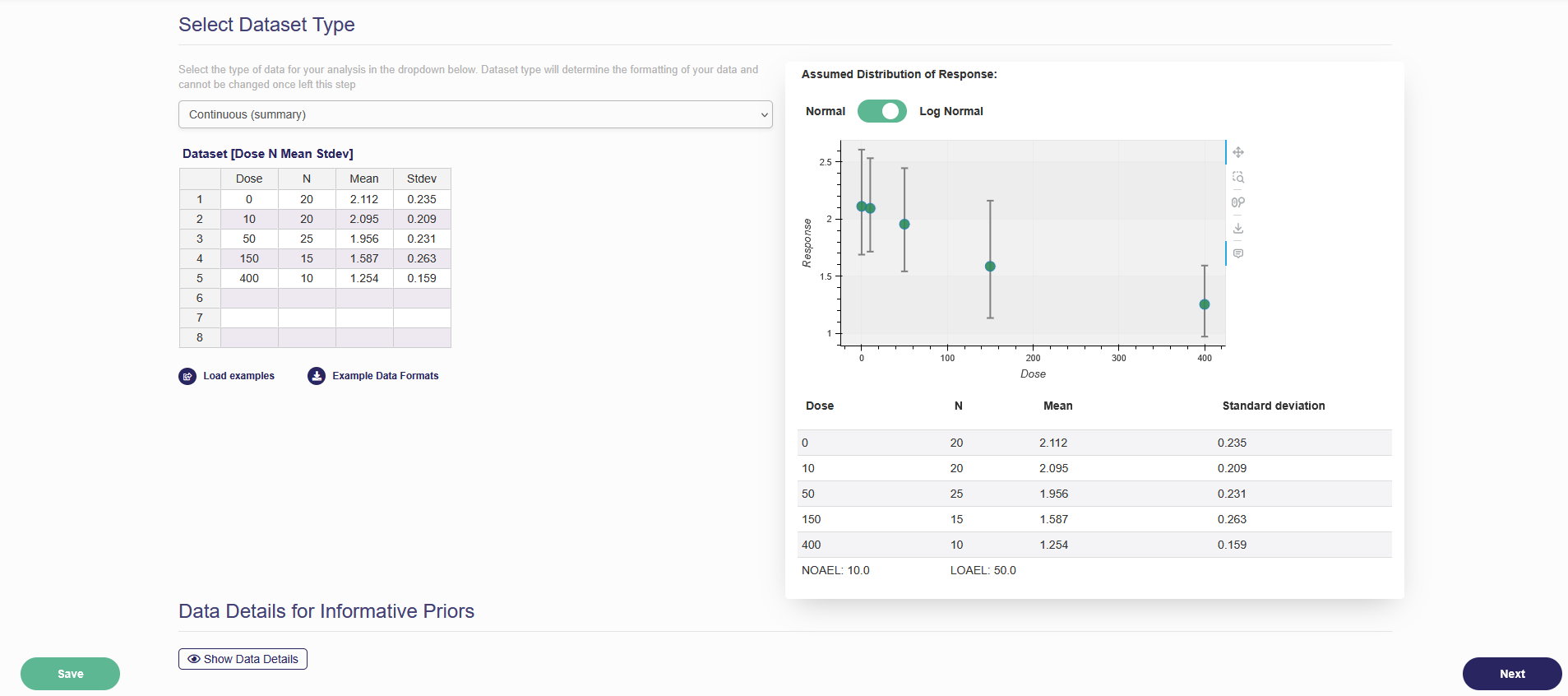
Figure 2.3. Data input page after inputting data

In addition to the table and the dose-response plot, If you uploaded continuous data, a trend test is performed. A p-value and z-score will be reported below the data table. The trend test results can be used to judge if the continuous dataset is appropriate for BMD modeling. Additionally, the NOAEL and LOAEL values will also be displayed. If you uploaded dichotomous data, a trend test (using the Cochran-Armitage linear trend test, same as the BMDS) is performed. A p-value and z-score will be reported below the data table. The trend test results can be used to judge if the dichotomous dataset is appropriate for BMD modeling. The NOAEL and LOAEL values will also be displayed. If you uploaded categorical data, the NOAEL and LOAEL values for each severity (i.e., category) will be displayed.

To continue to the next tab, press “Next” in the lower right corner.

C. MCMC Settings

On this tab (shown in Figure 2.4), you can specify some settings for the MCMC algorithms.

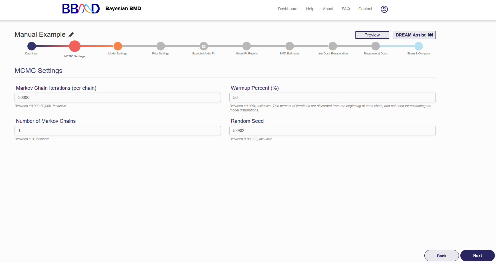
Figure 2.4. MCMC settings

How to make and change settings

 

There are four different values that need to be specified in this tab. First, specify the number of Markov chain iterations, between 10,000 and 50,000 (inclusive) iterations per chain. Enter your value into the “Markov Chain Iterations” text box. Next, you need to specify the warmup percentage for each Markov Chain. This is the percentage of iterations discarded from the beginning of each chain; Therefore, those iterations will not be used for estimating model distributions. Put this percentage in the “Warmup Percent (%)” text box. Third, specify the number of Markov chains used in the analysis. Enter a number 1 to 3 (inclusive) into the “Number of Markov Chains” text box. Each chain will use the number of iterations previously specified. The final value is the random seed which is used for reproducing analysis results. The random seed can be 0 to 99,999 (inclusive). Enter this value in the “Random Seed text box”.

Once these values are specified, click “Next” to save the MCMC settings and move to “Model Settings”. Default settings are generally acceptable. However, results in the next step will provide important information that can help you judge if the MCMC settings are appropriate. Based on our testing, the default settings are adequate for most of the commonly seen dose-response shapes, so we suggest you use the default settings for your initial run.

How MCMC settings may impact the results

 

“Iterations” is the length of MCMC chain, i.e., the number of posterior samples in each MCMC chain. Default value is 30,000. The allowable range is any integer between 10,000 and 50,000.

 

“Number of chains” is the number of Markov Chains to be sampled. Default value is 1. Allowable range is 1 - 3.

 

“Warmup percent (%)”, the percent of sample in each Markov Chain will be discarded from the final posterior sample. Default value is 50% with an allowable range of 10% - 90%.

 

So, using the default values, the final number of posterior sample (without the warmup sample) you can get is:

30000 × 1 × (1 − 50%) = 15000

“Seed” is random seed number used in the MCMC algorithms. The number is randomly generated, but you can specify the number for the purpose of reproduction.

D. Model Settings

Once data input and MCMC settings are completed, click “Next” to go to the next tab, “Model settings”. In this step, you should choose the model(s) to fit the data. To add a dose-response model, click the plus icon and then click “Create Model” or “Standard Models” on the left panel, shown in Figure 2.5. “Standard Models” includes all default models for each type of data which are described in section i-iii. 

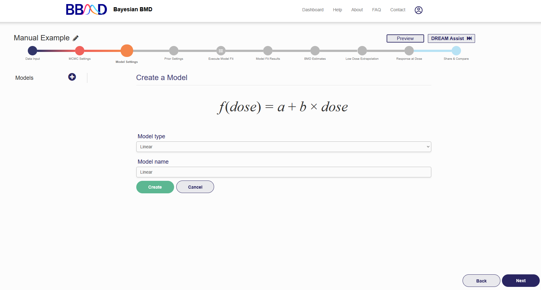
Figure 2.5. “Model Settings” tab

Follow these four steps to add a dose-response model to the list of models for the analysis:

1. Click the plus button in the left panel
2. Click “Create Model” in the box that appears
3. Select one model from the pull-down menu, then give an identifiable name to the model. For models with a power parameter, you need to choose a restriction value for the power parameter. There are five options available in the current system: 0, 0.25, 0.5, 0.75, and 1. The default value is 1.
4. Press the “Create” button to add the model to the list of models on the left panel.

To add another model, repeat the steps 1) to 4). The same model with different settings (e.g., the restriction value put on the power parameter) can be added again as a separate model.

To update a model from the model list, follow these 3 steps:

1. Click the three dots next name of the model you want to update or delete in the list of models on the left panel.
2. If you want to change the current settings of the model, click “Edit Model”, then you can modify the model settings like model type, model name, and the restriction value
3. Click “Update” below the settings to update the setting

You can delete a model which is already in the list of models by clicking the three dots next to the model’s name, and then clicking “Delete Model” and “Delete” in the window that pops up (Figure 2.6).

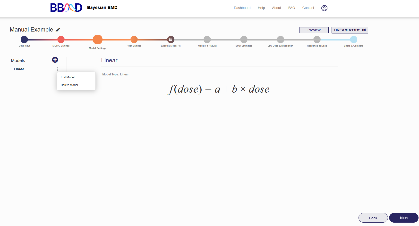
Figure 2.6. Update or Delete a Model in the List

Additionally, for both continuous and dichotomous data, you can choose to use empirical informative priors for the model parameters derived from the general database in Prior Settings. The default setting is the option “Non-Informative Prior” for the model(s) you have selected, which is followed by two options: “Empirical Informative Prior” and “Data Driven Informative Prior”. To turn informative priors on, select “Empirical Informative Prior”. The model(s) you choose to fit the data in Model Settings will be listed in the left panel. When specifying a model in the left panel, empirical prior distribution for each parameter in that model will be displayed. You can edit the parameters of the prior distribution such as mu and sigma for a normal distribution, or beta and alpha for the beta, and gamma distributions based on the recommended ranges shown below after clicking the three dots icon next to the model name and selecting “Edit Model”. Once the distributions are set, distribution curves for the parameters will also be displayed with the dose-response model formula, as shown in Figure 2.7. Currently, the option “Data Driven Informative Prior” is inactivated.

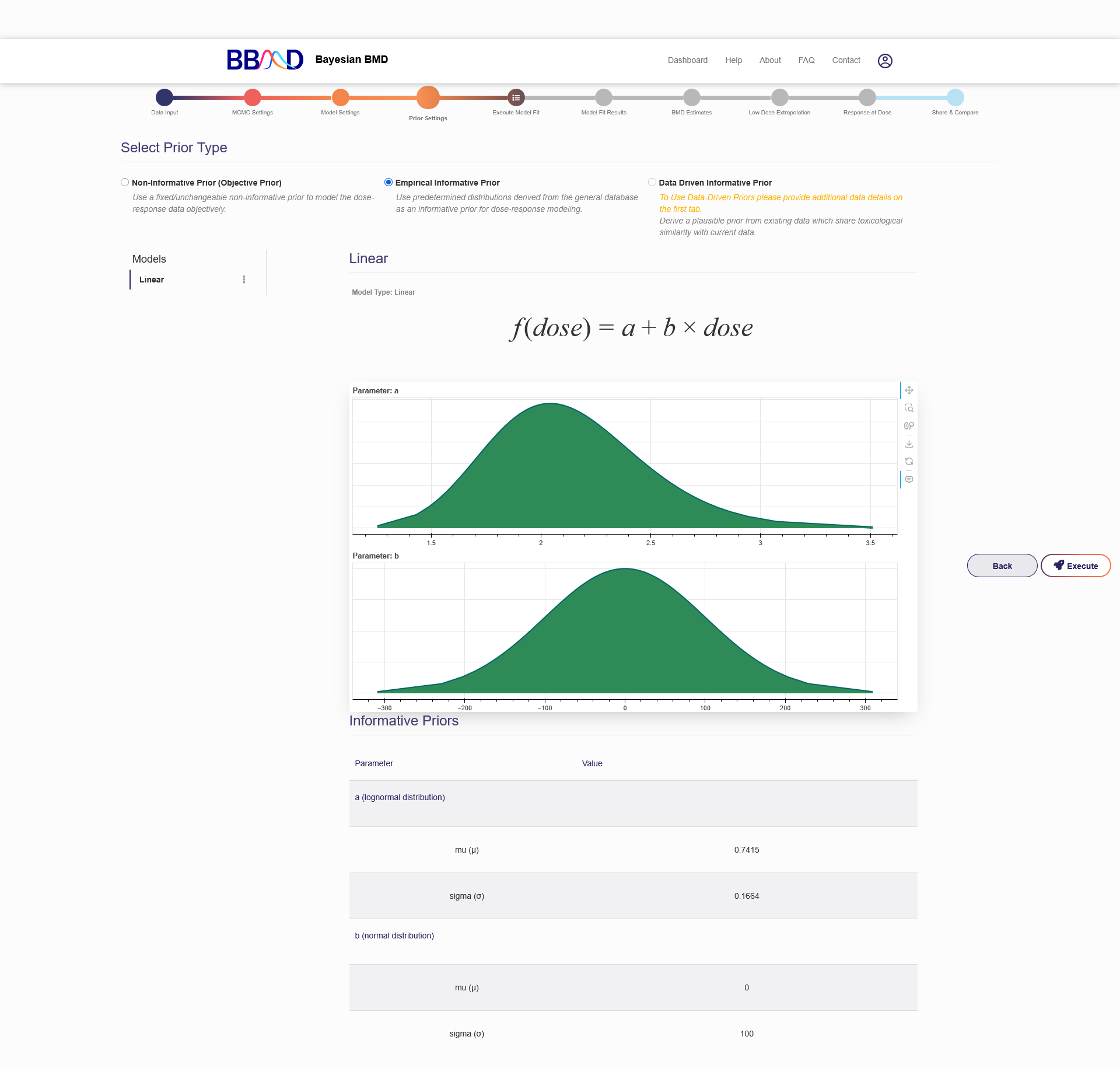
Figure 2.7. Distribution curves for dose-response model’s informative priors

When you keep the default setting, non-informative prior distribution is used as the default distribution for all the dose-response model parameters. The non-informative prior distributions for each model are listed below:

Dose-Response Models for Dichotomous Data

For Dichotomous data, there are eight models.

1) Quantal Linear Model:
𝑓(𝑑𝑜𝑠𝑒) = 𝑎 + (1 − 𝑎) × (1 − 𝑒^−𝑏×𝑑𝑜𝑠𝑒 )
𝑎~𝑈𝑛𝑖𝑓𝑜𝑟𝑚(0, 1); 𝑏~𝑈𝑛𝑖𝑓𝑜𝑟𝑚(0, 100)

2) Probit Model:
𝑓(𝑑𝑜𝑠𝑒) = 𝛷(𝑎 + 𝑏 × 𝑑𝑜𝑠𝑒)
𝑎~𝑈𝑛𝑖𝑓𝑜𝑟𝑚(−50, 50); 𝑏~𝑈𝑛𝑖𝑓𝑜𝑟𝑚(0, 100)

3) Logistic Model:
𝑓(𝑑𝑜𝑠𝑒) = 1/1 + 𝑒^(−𝑎−𝑏×𝑑𝑜𝑠𝑒)
𝑎~𝑈𝑛𝑖𝑓𝑜𝑟𝑚(−50, 50); 𝑏~𝑈𝑛𝑖𝑓𝑜𝑟𝑚(0, 100)

4) Weibull Model:
𝑓(𝑑𝑜𝑠𝑒) = 𝑎 + (1 − 𝑎) × (1 − 𝑒−𝑐×𝑑𝑜𝑠𝑒^𝑏)
𝑎~𝑈𝑛𝑖𝑓𝑜𝑟𝑚(0, 1); 𝑏~𝑈𝑛𝑖𝑓𝑜𝑟𝑚(0, 50); 𝑏~𝑈𝑛𝑖𝑓𝑜𝑟𝑚(𝑟𝑒𝑠𝑡𝑟𝑖𝑐𝑡𝑖𝑜𝑛, 15)
Where ‘restriction’ is a user defined value and can be 0, 0.25, 0.5, 0.75 or 1.

5) Multistage (2nd Order) Model:
𝑓(𝑑𝑜𝑠𝑒) = 𝑎 + (1 − 𝑎) × (1 − 𝑒−𝑏×𝑑𝑜𝑠𝑒−𝑐×𝑑𝑜𝑠𝑒^2)
𝑎~𝑈𝑛𝑖𝑓𝑜𝑟𝑚(0, 1); 𝑏~𝑈𝑛𝑖𝑓𝑜𝑟𝑚(0, 100); 𝑐~𝑈𝑛𝑖𝑓𝑜𝑟𝑚(0, 100)

6) LogLogistic Model:
𝑓(𝑑𝑜𝑠𝑒) = 𝑎 + (1 − 𝑎)/(1 + 𝑒−𝑐−𝑏×𝑙𝑜𝑔(𝑑𝑜𝑠𝑒))
𝑎~𝑈𝑛𝑖𝑓𝑜𝑟𝑚(0, 1); 𝑏~𝑈𝑛𝑖𝑓𝑜𝑟𝑚(𝑟𝑒𝑠𝑡𝑟𝑖𝑐𝑡𝑖𝑜𝑛, 15); 𝑐~𝑈𝑛𝑖𝑓𝑜𝑟𝑚(−5, 15)

7) LogProbit Model:
𝑓(𝑑𝑜𝑠𝑒) = 𝑎 + (1 − 𝑎) × 𝛷(𝑐 + 𝑏 × 𝑙𝑜𝑔(𝑑𝑜𝑠𝑒))
𝑎~𝑈𝑛𝑖𝑓𝑜𝑟𝑚(0, 1); 𝑏~𝑈𝑛𝑖𝑓𝑜𝑟𝑚(𝑟𝑒𝑠𝑡𝑟𝑖𝑐𝑡𝑖𝑜𝑛, 15); 𝑐~𝑈𝑛𝑖𝑓𝑜𝑟𝑚(−5, 15)

8) Dichotomous Hill Model:
𝑓(𝑑𝑜𝑠𝑒) = 𝑎 × 𝑔 + (𝑎 − 𝑎 × 𝑔)/(1 + 𝑒^−𝑐−𝑏×𝑙𝑜𝑔(𝑑𝑜𝑠𝑒))
𝑎~𝑈𝑛𝑖𝑓𝑜𝑟𝑚(0, 1); 𝑏~𝑈𝑛𝑖𝑓𝑜𝑟𝑚(𝑟𝑒𝑠𝑡𝑟𝑖𝑐𝑡𝑖𝑜𝑛, 15); 𝑐~𝑈𝑛𝑖𝑓𝑜𝑟𝑚(−5, 15); 𝑔~𝑈𝑛𝑖𝑓𝑜𝑟𝑚(0, 1)

These eight models are also the models which are part of the “Standard Models” for Dichotomous data.

Dose-Response Models for Continuous Data

Background parameter ‘a’

The background parameter “a” in all eight models has the same uniform distribution used as prior which is derived as follow:

The lower bound of the uniform distribution is always 0, and the upper bound is calculated differently for individual data and summary data.

For individual data,

𝑎_𝑢𝑝𝑝𝑒𝑟 = max (𝑟𝑒𝑠𝑝𝑜𝑛𝑠𝑒) × 2

i.e., doubling the largest response value in the input dataset.

For summary data,

𝑎_𝑢𝑝𝑝𝑒𝑟 = (max(𝑟𝑒𝑠𝑝. 𝑚𝑒𝑎𝑛) + 2 × 𝑟𝑒𝑠𝑝. 𝑠𝑑_𝑚𝑒𝑎𝑛.𝑚𝑎𝑥) × 2

Where max(𝑟𝑒𝑠𝑝. 𝑚𝑒𝑎𝑛) is the maximum mean response across all dose groups in the input dataset, and 𝑟𝑒𝑠𝑝. 𝑠𝑑𝑚𝑒𝑎𝑛.𝑚𝑎𝑥 is the response standard deviation in that dose group with the maximum mean response.

Slope parameter 'b'

For the Linear, Power, Michaelis Menten and Hill model, the lower or upper bound of the parameter b (a slope-equivalent parameter) are determined by the dose-response trend and the overall slope in the input data.

For individual input data and increasing trend:

𝑏_𝑙𝑜𝑤𝑒𝑟 = 0

𝑏_𝑢𝑝𝑝𝑒𝑟 = (𝑀𝑎𝑥(𝑟𝑒𝑠𝑝) − 𝑀𝑖𝑛(𝑟𝑒𝑠𝑝))/(𝐷𝑜𝑠𝑒_𝑀𝑎𝑥_𝑟𝑒𝑠𝑝 − 𝐷𝑜𝑠𝑒_𝑀𝑖𝑛_𝑟𝑒𝑠𝑝)× 5

For individual input data and decreasing trend:

𝑏_𝑙𝑜𝑤𝑒𝑟 = (𝑀𝑖𝑛(𝑟𝑒𝑠𝑝) − 𝑀𝑎𝑥(𝑟𝑒𝑠𝑝)) / (𝐷𝑜𝑠𝑒_𝑀𝑖𝑛_𝑟𝑒𝑠𝑝 − 𝐷𝑜𝑠𝑒_𝑀𝑎𝑥_𝑟𝑒𝑠𝑝) × 5
𝑏𝑢𝑝𝑝𝑒𝑟 = 0

Where 𝑀𝑎𝑥(𝑟𝑒𝑠𝑝) and 𝑀𝑖𝑛(𝑟𝑒𝑠𝑝) are the maximum and minimum response value in the input dataset. And 𝐷𝑜𝑠𝑒𝑀𝑎𝑥_𝑟𝑒𝑠𝑝 and 𝐷𝑜𝑠𝑒𝑀𝑖𝑛_𝑟𝑒𝑠𝑝 are the dose levels corresponding to the maximum and minimum responses respectively.

For summary input data:
𝑏𝑠𝑙𝑜𝑝𝑒 = (𝑀𝑒𝑎𝑛_𝑀𝑎𝑥_𝑑𝑜𝑠𝑒 + 2 × 𝑆𝐷_𝑀𝑎𝑥_𝑑𝑜𝑠𝑒 −𝑀𝑒𝑎𝑛_𝑀𝑖𝑛_𝑑𝑜𝑠𝑒 − 2 × 𝑆𝐷_𝑀𝑖𝑛_𝑑𝑜𝑠𝑒)/(𝑀𝑎𝑥(𝑑𝑜𝑠𝑒) − 𝑀𝑖𝑛(𝑑𝑜𝑠𝑒))

Where 𝑀𝑒𝑎𝑛_𝑀𝑎𝑥_𝑑𝑜𝑠𝑒 and 𝑆𝐷_𝑀𝑎𝑥_𝑑𝑜𝑠𝑒 are the mean and standard deviation of responses at the maximum dose level, and 𝑀𝑒𝑎𝑛𝑀𝑖𝑛_𝑑𝑜𝑠𝑒 and 𝑆𝐷𝑀𝑖𝑛_𝑑𝑜𝑠𝑒 are the mean and standard deviation of responses at the minimum dose level. 𝑀𝑎𝑥(𝑑𝑜𝑠𝑒) and 𝑀𝑖𝑛(𝑑𝑜𝑠𝑒) are the maximum and minimum dose levels in the input dataset. Because dose levels are first normalized to the scale between 0 and 1, 𝑀𝑎𝑥(𝑑𝑜𝑠𝑒) is very likely 1 and 𝑀𝑖𝑛(𝑑𝑜𝑠𝑒) is very likely 0. Then the prior distribution of the parameter “s” is 𝑈𝑛𝑖𝑓𝑜𝑟𝑚(0, 5 × 𝑏𝑠𝑙𝑜𝑝𝑒) for increasing trend and 𝑈𝑛𝑖𝑓𝑜𝑟𝑚(5 × 𝑏𝑠𝑙𝑜𝑝𝑒 , 0) for decreasing trend.

For continuous data, there are eight models.

1) Linear Model:
𝑓(𝑑𝑜𝑠𝑒) = 𝑎 + 𝑏 × 𝑑𝑜𝑠𝑒
𝑎~𝑈𝑛𝑖𝑓𝑜𝑟𝑚(0, 𝑎_𝑢𝑝𝑝𝑒𝑟); 𝑏~𝑈𝑛𝑖𝑓𝑜𝑟𝑚(𝑏_𝑙𝑜𝑤𝑒𝑟, 𝑏_𝑢𝑝𝑝𝑒𝑟)

2) Power Model:
𝑓(𝑑𝑜𝑠𝑒) = 𝑎 + 𝑏 × 𝑑𝑜𝑠𝑒𝑔
𝑎~𝑈𝑛𝑖𝑓𝑜𝑟𝑚(0, 𝑎_𝑢𝑝𝑝𝑒𝑟); 𝑏~𝑈𝑛𝑖𝑓𝑜𝑟𝑚(𝑏_𝑙𝑜𝑤𝑒𝑟, 𝑏_𝑢𝑝𝑝𝑒𝑟); 𝑔~𝑈𝑛𝑖𝑓𝑜𝑟𝑚(𝑟𝑒𝑠𝑡𝑟𝑖𝑐𝑡𝑖𝑜𝑛, 15)
Where ‘restriction’ is a user defined value and can be 0, 0.25, 0.5, 0.75 or 1.

3) Michaelis-Menten Model:
𝑓(𝑑𝑜𝑠𝑒) = 𝑎 + 𝑏 × 𝑑𝑜𝑠𝑒
𝑐 + 𝑑𝑜𝑠𝑒
𝑎~𝑈𝑛𝑖𝑓𝑜𝑟𝑚(0, 𝑎_𝑢𝑝𝑝𝑒𝑟); 𝑏~𝑈𝑛𝑖𝑓𝑜𝑟𝑚(𝑏_𝑙𝑜𝑤𝑒𝑟, 𝑏_𝑢𝑝𝑝𝑒𝑟); 𝑐~𝑈𝑛𝑖𝑓𝑜𝑟𝑚(0, 15)

4) Hill Model:
𝑓(𝑑𝑜𝑠𝑒) = 𝑎 + (𝑏 × 𝑑𝑜𝑠𝑒^𝑔)/(𝑐^𝑔 + 𝑑𝑜𝑠𝑒^𝑔)
𝑎~𝑈𝑛𝑖𝑓𝑜𝑟𝑚(0, 𝑎𝑢𝑝𝑝𝑒𝑟); 𝑏~𝑈𝑛𝑖𝑓𝑜𝑟𝑚(𝑏𝑙𝑜𝑤𝑒𝑟, 𝑏𝑢𝑝𝑝𝑒𝑟); 𝑐~𝑈𝑛𝑖𝑓𝑜𝑟𝑚(0, 15); 𝑔~𝑈𝑛𝑖𝑓𝑜𝑟𝑚(𝑟𝑒𝑠𝑡𝑟𝑖𝑐𝑡𝑖𝑜𝑛, 15);
where ‘restriction’ is a user defined value and can be 0, 0.25, 0.5, 0.75 or 1.

5) Exponential 2 Model:
𝑓(𝑑𝑜𝑠𝑒) = 𝑎 × 𝑒^(𝑏×𝑑𝑜𝑠𝑒)
𝑎~𝑈𝑛𝑖𝑓𝑜𝑟𝑚(0, 𝑎𝑢𝑝𝑝𝑒𝑟); 𝑏~𝑈𝑛𝑖𝑓𝑜𝑟𝑚(0, 50) for increasing trend or 𝑈𝑛𝑖𝑓𝑜𝑟𝑚(−50, 0) for decreasing trend.

6) Exponential 3 Model:
(𝑑𝑜𝑠𝑒) = 𝑎 × 𝑒^(𝑏×𝑑𝑜𝑠𝑒^𝑔)
𝑎~𝑈𝑛𝑖𝑓𝑜𝑟𝑚(0, 𝑎_𝑢𝑝𝑝𝑒𝑟);
𝑏~𝑈𝑛𝑖𝑓𝑜𝑟𝑚(0, 50) for increasing trend or 𝑈𝑛𝑖𝑓𝑜𝑟𝑚(−50, 0) for decreasing trend;
𝑔~𝑈𝑛𝑖𝑓𝑜𝑟𝑚(𝑟𝑒𝑠𝑡𝑟𝑖𝑐𝑡𝑖𝑜𝑛, 15);
where ‘restriction’ is a user defined value and can be 0, 0.25, 0.5, 0.75 or 1.

7) Exponential 4 Model:
𝑓(𝑑𝑜𝑠𝑒) = 𝑎 × (𝑐 − (𝑐 − 1) × 𝑒^(−𝑏×𝑑𝑜𝑠𝑒 ))
𝑎~𝑈𝑛𝑖𝑓𝑜𝑟𝑚(0, 𝑎𝑢𝑝𝑝𝑒𝑟); 𝑏~𝑈𝑛𝑖𝑓𝑜𝑟𝑚(0, 100); 𝑐~𝑈𝑛𝑖𝑓𝑜𝑟𝑚(0, 1) for decreasing trend or 𝑐~𝑈𝑛𝑖𝑓𝑜𝑟𝑚(1, 15) for increasing trend.

8) Exponential 5 Model:
𝑓(𝑑𝑜𝑠𝑒) = 𝑎 × (𝑐 − (𝑐 − 1) × 𝑒^−(𝑏×𝑑𝑜𝑠𝑒)^𝑔)
𝑎~𝑈𝑛𝑖𝑓𝑜𝑟𝑚(0, 𝑎𝑢𝑝𝑝𝑒𝑟); 𝑏~𝑈𝑛𝑖𝑓𝑜𝑟𝑚(0, 100); 𝑐~𝑈𝑛𝑖𝑓𝑜𝑟𝑚(0, 15) for decreasing trend or 𝑐~𝑈𝑛𝑖𝑓𝑜𝑟𝑚(1, 15) for increasing trend; 𝑔~𝑈𝑛𝑖𝑓𝑜𝑟𝑚(𝑟𝑒𝑠𝑡𝑟𝑖𝑐𝑡𝑖𝑜𝑛, 15);
where ‘restriction’ is a user defined value and can be 0, 0.25, 0.5, 0.75 or 1.

For continuous data, all eight of these models are included in the “Standard Models”

Dose-Response Models for Categorical Data

1) Logistic Model:
𝑓(𝑑𝑜𝑠𝑒) = 1/(1 + 𝑒^(−𝑎−𝑏×𝑑𝑜𝑠𝑒))
𝑎~𝑈𝑛𝑖𝑓𝑜𝑟𝑚(−50, 50); 𝑏~𝑈𝑛𝑖𝑓𝑜𝑟𝑚(0, 100)

2) Probit Model:
𝑓(𝑑𝑜𝑠𝑒) = 𝛷(𝑎 + 𝑏 × 𝑑𝑜𝑠𝑒), 𝑏 ≥ 0
𝑎~𝑈𝑛𝑖𝑓𝑜𝑟𝑚(−50, 50); 𝑏~𝑈𝑛𝑖𝑓𝑜𝑟𝑚(0, 50)

3) Cloglog Model:
𝑓(𝑑𝑜𝑠𝑒) = 1 − 𝑒^−𝑒^(𝑎+𝑏×𝑑𝑜𝑠𝑒)
𝑎~𝑈𝑛𝑖𝑓𝑜𝑟𝑚(−100, 100); 𝑏~𝑈𝑛𝑖𝑓𝑜𝑟𝑚(0, 100)

4) Quantal Linear Model:
𝑓(𝑑𝑜𝑠𝑒) = 𝑎 + (1 − 𝑎) × (1 − 𝑒^(−𝑏×𝑑𝑜𝑠𝑒 ))
𝑎~𝑈𝑛𝑖𝑓𝑜𝑟𝑚(0, 1); 𝑏~𝑈𝑛𝑖𝑓𝑜𝑟𝑚(0, 100)

5) Multistage (2nd Order) Model:
𝑓(𝑑𝑜𝑠𝑒) = 𝑎 + (1 − 𝑎) × (1 − 𝑒^(−𝑏×𝑑𝑜𝑠𝑒−𝑐×𝑑𝑜𝑠𝑒^2))
𝑎~𝑈𝑛𝑖𝑓𝑜𝑟𝑚(0, 1); 𝑏~𝑈𝑛𝑖𝑓𝑜𝑟𝑚(0, 100); 𝑐~𝑈𝑛𝑖𝑓𝑜𝑟𝑚(0, 100)

6) Weibull Model:
𝑓(𝑑𝑜𝑠𝑒) = 𝑎 + (1 − 𝑎) × (1 − 𝑒^(−𝑐×𝑑𝑜𝑠𝑒^𝑏))
𝑎~𝑈𝑛𝑖𝑓𝑜𝑟𝑚(0, 1); 𝑏~𝑈𝑛𝑖𝑓𝑜𝑟𝑚(𝑟𝑒𝑠𝑡𝑟𝑖𝑐𝑡𝑖𝑜𝑛, 15); 𝑐~𝑈𝑛𝑖𝑓𝑜𝑟𝑚(0, 50);
where ‘restriction’ is a user defined value and can be 0, 0.25, 0.5, 0.75 or 1.

7) LogLogistic Model:
𝑓(𝑑𝑜𝑠𝑒) = 𝑎 + (1 − 𝑎)/(1 + 𝑒^(−𝑐−𝑏×𝑙𝑜𝑔(𝑑𝑜𝑠𝑒)))
𝑎~𝑈𝑛𝑖𝑓𝑜𝑟𝑚(0, 1); 𝑏~𝑈𝑛𝑖𝑓𝑜𝑟𝑚(𝑟𝑒𝑠𝑡𝑟𝑖𝑐𝑡𝑖𝑜𝑛, 15); 𝑐~𝑈𝑛𝑖𝑓𝑜𝑟𝑚(−5, 15);
where ‘restriction’ is a user defined value and can be 0, 0.25, 0.5, 0.75 or 1.

8) LogProbit Model:
𝑓(𝑑𝑜𝑠𝑒) = 𝑎 + (1 − 𝑎) × 𝛷(𝑐 + 𝑏 × 𝑙𝑜𝑔(𝑑𝑜𝑠𝑒))
𝑎~𝑈𝑛𝑖𝑓𝑜𝑟𝑚(0, 1); 𝑏~𝑈𝑛𝑖𝑓𝑜𝑟𝑚(𝑟𝑒𝑠𝑡𝑟𝑖𝑐𝑡𝑖𝑜𝑛, 15); 𝑐~𝑈𝑛𝑖𝑓𝑜𝑟𝑚(−5, 15);
where ‘restriction’ is a user defined value and can be 0, 0.25, 0.5, 0.75 or 1.

These eight models are available to be used as dose-response models for categorical data, but the “Standard Models” are reduced to the Logistic, Probit, and Cloglog models.

The models shown on the left panel are the models will be analyzed by the system. Once you are happy with the models selected and the model settings, click “Execute” in the bottom right corner to execute model fitting.

E. Model Fit Results

On the “Model Fit Results” tab, the model fitting results obtained from the previous step are displayed. Click the name of one of the models on the left panel, then the results will be shown on the right (as shown in Figure 2.8) These results include the textual output of model parameter estimation, dynamic dose-response plot, posterior predictive p-value, model weight, correlation matrix, and graphical output of posterior sample of the model parameters (hidden by default). When click “Hide Parameters”, the parameter charts for each parameter in the model are displayed as shown in Figure 2.9.

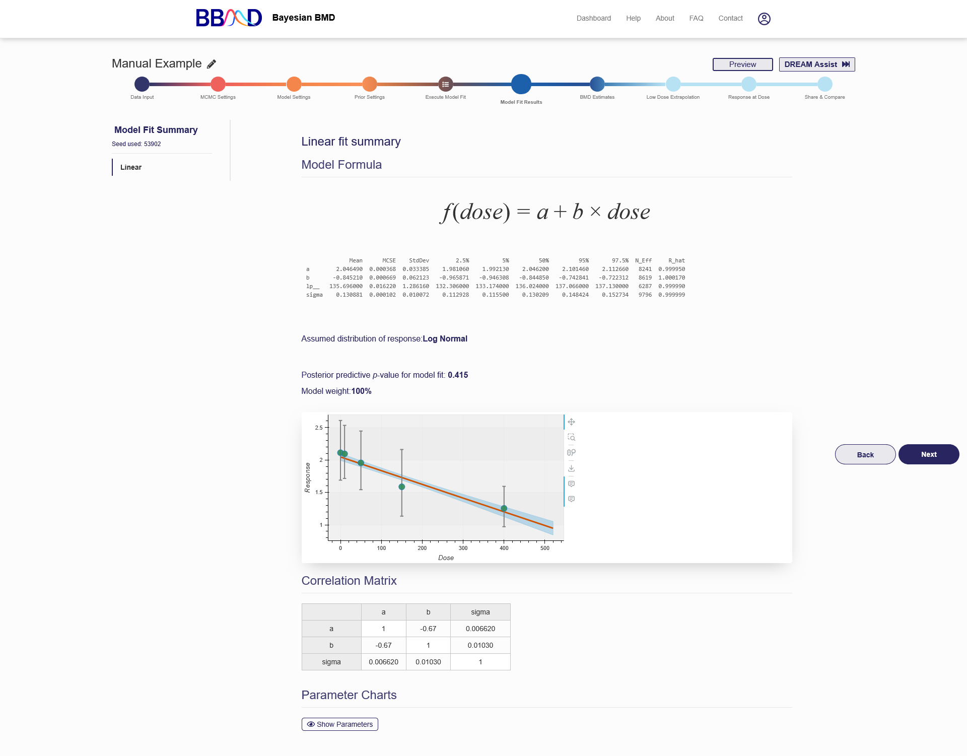
Figure 2.8. Results Shown on the “Model fit Results” Page

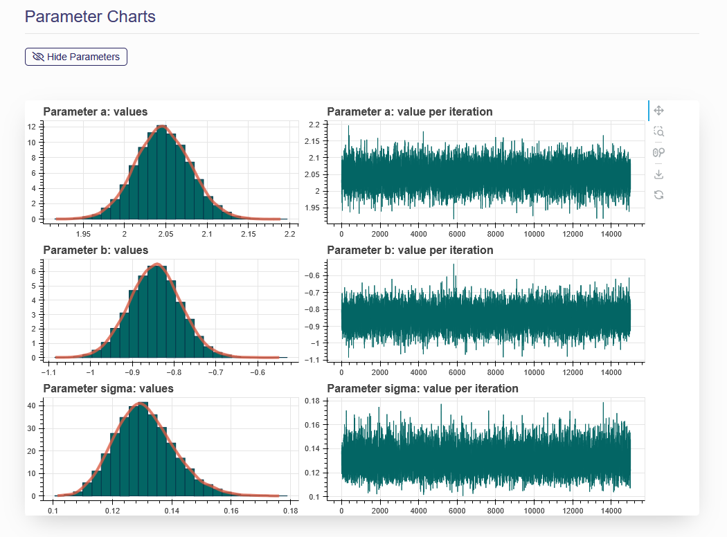
Figure 2.9. Parameter Charts 

Parameter estimation results

The parameter estimation results, displayed in a table under the model formula, show the statistical summary for the estimated posterior distributions of parameters in the given dose-response model. These results are obtained directly from PyStan’s fit output, including some important statistics for model parameters and diagnostic indictors for the MCMC algorithms. The mean, standard error of the mean (MCSE), standard deviation (StdDev), various quantiles (2.5%, 25%, 50%, 75%, and 97.5%), and quantities indicating effective sample size (N_Eff) and chain convergence (Rhat) for each model parameter derived from the posterior distribution of each parameter, as well as information regarding the MCMC execution are summarized in the table. As a note, the “Rhat” can be used to judge if the MCMC chains have converged properly. If the Rhat value is larger than 1.05, you may consider increasing the length of MCMC chains to get better convergence. 

Posterior Predictive P-Value

A posterior predictive p-value (PPP value) is reported below the dynamic dose-response plot. The PPP can be approximated by counting the predicted responses that satisfy the inequality out of the entire posterior sample space. This indicator can be used to judge if the fitting of this particular model is adequate. A large or small p-value means that a discrepancy in predicted data is very likely, further indicating a poor fit. Practically, if the PPP value is between 0.05 and 0.95, then the fitting is adequate. The calculation procedure of PPP value is briefly described below:

1. Use each bundle of parameters in the kept posterior sample to form a dose-response model and randomly generate case numbers, 𝑦^𝑟𝑒𝑝, at all dose levels in the original dataset
2. Use posterior sample of model parameters to calculate a test statistic for both the original data set (𝑑, 𝑛, 𝑦) and the replicated data set (𝑑, 𝑛, 𝑦^𝑟𝑒𝑝). The test statistic used in this system is log-likelihood. For parameter values from l-th iteration, we have statistic 𝑇(𝑦, 𝜃^𝑙) and 𝑇(𝑦^𝑟𝑒𝑝, 𝜃^𝑙).
3. For l = 1, …, L (the length of posterior sample), compare each pair of 𝑇(𝑦, 𝜃^𝑙 ) and 𝑇(𝑦^𝑟𝑒𝑝, 𝜃^𝑙), and count the number of 𝑇(𝑦, 𝜃^𝑙) > 𝑇(𝑦^𝑟𝑒𝑝, 𝜃^𝑙), say 𝑀
4. The posterior predictive P-value is 𝑀/𝐿

A detailed explanation on this procedure can be found in the Chapter of “Model checking and improvement” in Bayesian Data Analysis (Gelman et al).

Posterior Model Weight

A model weight (𝑚̂_𝑗) for model j is calculated for each model included in the analysis as a statistic for cross-model comparison. The model weight was introduced by (Wasserman, 2000), using the following two equations. The 𝑚̂_𝑗 value of each selected model j is calculated as follows:

𝑚̂_𝑗 = exp (ℓ̂_𝑗 − (𝑑_𝑗/2)×𝑙𝑜𝑔(𝑛))

where ℓ̂_𝑗 is a loglikelihood value estimated using one set of posterior samples of model parameters of the jth model, 𝑑_𝑗 is number of parameters in the jth model, and 𝑛 is the sample size in the data set.

When all models in the analysis have an equal prior weight, the posterior model weight of model j is calculated by m value estimated from model j divided by the sum of m values estimated from all models in the analysis as the following equation.

Pr(ℳ_𝑗|𝐷𝑎𝑡𝑎) = 𝑚̂_𝑗/∑ 𝑚̂_t

This function assumes equal model priors for all models selected, so the weight mainly indicates how well the model fits the data. To make the weight more reliable, we use 1000 sets of randomly selected posterior samples of model parameters to calculate the model weights. This model weights are further applied to the model averaged BMD calculation in the F. BMD Estimation section.

Interactive Dose-Response Plot

A dynamic dose-response plot is shown below the text box. This plot includes original dose-response data and a fitted curve with its 90th percentile interval shaded in blue. When you move your mouse over the dose-response curve, the estimated median and the 5th and 95th percentiles at a particular dose level will display. When you move your mouse over a data point from your inputted dataset, the dose, N, incidence, and the response percentile will also be displayed. Other information displayed in this figure includes the PyStan version, the lower bound placed on the power parameter (if applicable), the posterior predictive p-value (PPP value) for model fit and model weight for cross-model comparison.  

Correlation Matrix

The fourth item displayed is the correlation matrix for the different model parameters. The correlation matrix is to show the correlation coefficients between different model parameters and is calculated using posterior samples. 

Plots for parameter posterior sample

 

If you click the “Show Parameters” under Parameter Charts, two plots (posterior sample trace plot and estimated probability density plot) will be displayed for each of the parameters in this dose-response model.

Basically, this is the results display tab, meaning that you can only review the results, not give the system additional inputs to modify the results.

F. BMD Estimation

On this page, you can calculate the BMD estimates of your interest. The settings for BMD calculation are slightly different between the analysis for dichotomous data, continuous data and categorical data, therefore, they will be introduced separately.

Dichotomous Data

Figure 2.10 is a screenshot of the “BMD estimates” tab for a dichotomous dataset. To create a BMD analysis, you need to follow the four steps below:

1. Name the BMD analysis using an easily identifiable name in the “BMD setting name” box.
2. Specify a BMR value in the “Benchmark response value” box.
3. Give prior model weight to the models included in this analysis. For your reference, “Additional Info” section provides you further info on the performances of each model fitting. The prior weight, PPP value and the calculated weights for each model are provided when you change the slider in the right side of the page below “Additional Info” to green. The prior weight will influence the estimation of model averaged BMD value. Giving 0 prior weight to a particular model can exclude the model from model-averaged BMD calculation. The sum of the weights assigned to the individual models are not necessarily required to be 1. The system will automatically convert them. For example, if you give 1 to Logistic model and 3 to Probit model, the system will convert these values to 25% prior weight for the Logistic model and 75% prior weight for the Probit model.
4. Click the “Execute” button to execute the BMD analysis using the settings just specified.

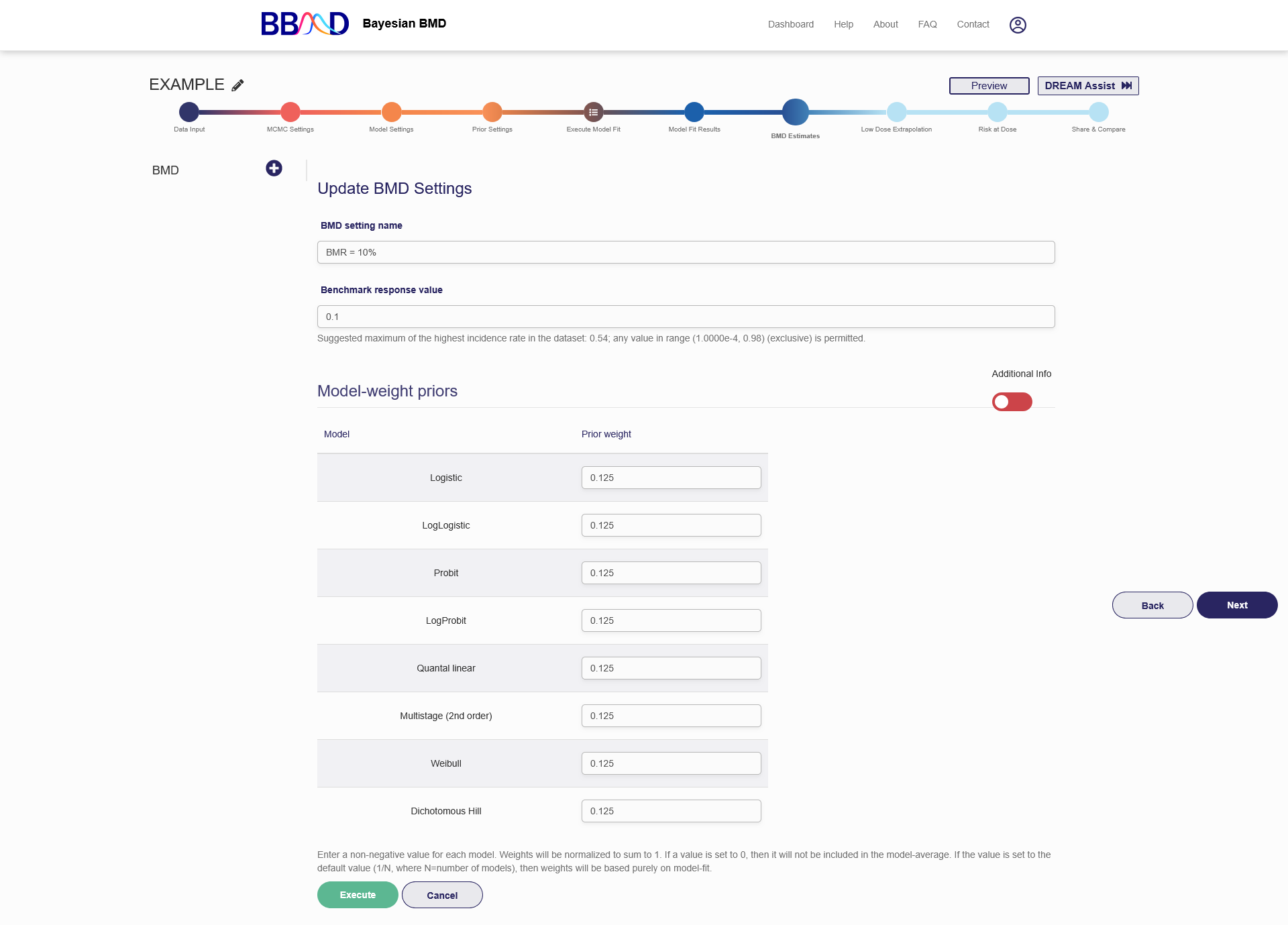
Figure 2.10. BMD Analysis Input for Dichotomous Data

Once the BMD analysis is successfully created, the name of the analysis will show on the left panel and the results will be displayed on the right panel, as shown in Figure 19. The results for a BMD analysis will include all the BMD distribution plots from each model, and a summary table. The estimation plots are shown in Figure 2.11, and the summary table is shown in Figure 2.12. To add a new BMD analysis, click the plus button in the left column and repeat steps (1) to (4) above. To edit or delete an existing BMD analysis, click the pencil in the upper right corner. From here you can change the name, BMR value, or model weights the same way as when the analysis was created. To save the changes made, click “Execute” on the bottom of the page. To delete this analysis, click “Delete”. To cancel the modification, click “Cancel”.

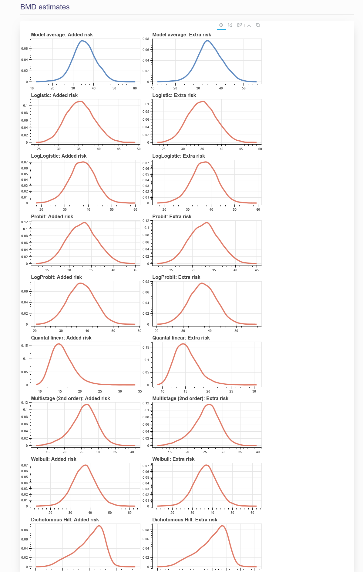
Figure 2.11. BMD Estimation plots from “BMD Estimates” tab

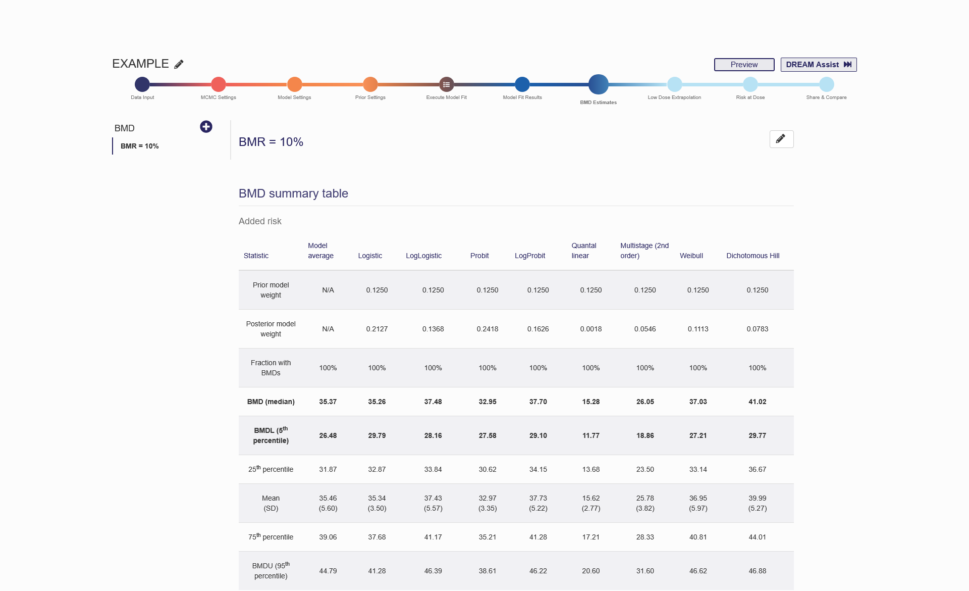
Figure 2.12. BMD Estimation Results Shown on the “BMD Estimates” tab

For dichotomous data, the BMD will be calculated for both the added risk and extra risk. For the two risks, the BMDs are defined by the following equations, respectively:

Added risk: 𝑓(𝐵𝑀𝐷) − 𝑓(0) = 𝐵𝑀𝑅, Extra risk: (𝑓(𝐵𝑀𝐷)−𝑓(0))/(1−𝑓(0)) = 𝐵𝑀𝑅;

where 𝑓(∙) represents a dichotomous dose–response model. BMR stands for benchmark response, which is a specified increase in the probability of response and is commonly set at 10%, 5%, or 1%.

In BBMD, the posterior distribution of BMD estimation is established. With the posterior sample, a number of statistics (including the mean, median, standard deviation, and other quantiles) of BMD can be computed and are reported in the “BMD summary table” on the “BMD Estimates” tab. Based on our testing, the median value of the BMD posterior sample is the most reliable estimate for BMD owing to its resistance to some extreme values in the sample. In addition, the 5th percentile of the posterior sample is considered the lower bound of BMD (i.e., BMDL) corresponding to the lower bound of the one-sided 95th confidence interval. The BMDL is usually used as the point of departure for low-dose extrapolation and is therefore of great regulatory interest. The BMD and BMDL values are highlighted in the “BMD summary table”. The same procedures used for determining BMD and BMDL are also applied to continuous and categorical data.

Continuous Data

For continuous data, the BBMD system provides two ways to define BMD: (1) based on central tendency and (2) based on tails (hybrid approach). The basic steps to create a BMD analysis for continuous data are almost identical to the procedure for dichotomous data, except the settings for the BMR. “Central tendency” is the default option for BMD estimation method of continuous data. 

Figure 2.13 is a screenshot of the “BMD Estimates” tab for a continuous dataset using Central tendency as the BMD estimation method. To create a BMD analysis, you need to follow the six steps below:

1. Name the BMD analysis using an easily identifiable name in the “BMD setting name” box.
2. Specify “Central Tendency” as the estimation method to be used in the “BMD estimation method” drop-down menu. If you wish to use “Hybrid Method (tails)”, the detailed steps are in the next section.
3. Select an adversity measure from the “Adversity measure” drop-down menu. For BMD defined on central tendency, there are three options for defining the BMR value: a) relative change, b) absolute change, and c) cutoff. Detailed explanations on the three options are in section b.
4. Specify an adversity value in the “Adversity value” text box.
5. Give prior model weight to the models included in this analysis. “Additional Info” section provides you further info on the performances of each model fitting. The prior weight, PPP value and the calculated weights for each model are provided when you change the slider in the right side of the page below “Additional Info” to green. The prior weight will influence the estimation of model averaged BMD value. Giving 0 weight to a particular model can exclude the model from model-averaged BMD calculation. The sum of the weights assigned to the individual models are not necessarily required to be 1. The system will automatically convert them. For example, if you give 1 to Linear model and 3 to Exponential 2 model, the system will convert these values to 25% prior weight for the Linear model and 75% prior weight for the Exponential 2 model.
6. Click the “Execute” button to execute the BMD analysis using the settings just specified.

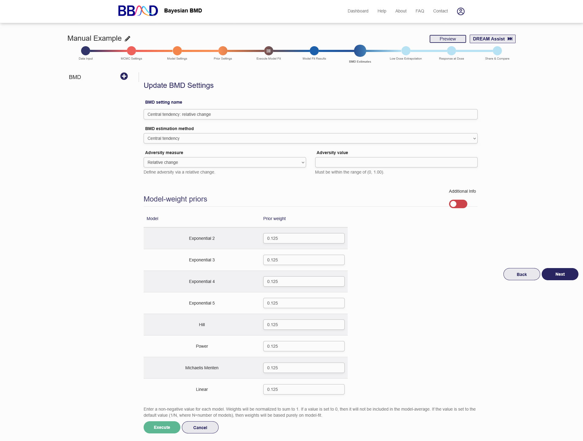
Figure 2.13. Settings for Continuous Data BMD Calculation Based on Central Tendency

 

Figure 2.14 is a screenshot of the “BMD Estimates” tab for a continuous dataset using the hybrid method (tails) as the estimation method. To create a BMD analysis, follow the seven steps below:

1. Name the BMD analysis using an easily identifiable name in the “BMD setting name” box.
2. Specify “Hybrid Method (tails)” as the estimation method to be used in the “BMD estimation method” drop-down menu.
3. Select an adversity measure from the “Adversity measure” drop-down menu. For BMD defined on hybrid method, there are two options for defining the BMR value: a) control group percentile, and b) absolute cutoff value.
4. Specify an adversity value in the “Adversity value” text box.
5. Specify a BMR value in the “Benchmark response value” text box.
6. Give prior model weight to the models included in this analysis. “Additional Info” section provides you further info on the performances of each model fitting. The prior weight, PPP value and the calculated weights for each model are provided when you change the slider in the right side of the page below “Additional Info” to green. The prior weight will influence the estimation of model averaged BMD value. Giving 0 weight to a particular model can exclude the model from model-averaged BMD calculation. The sum of the weights assigned to the individual models are not necessarily required to be 1. The system will automatically convert them. For example, if you give 1 to Linear model and 3 to Exponential 2 model, the system will convert these values to 25% prior weight for the Linear model and 75% prior weight for the Exponential 2 model.
7. Click the “Execute” button to execute the BMD analysis using the settings just specified.

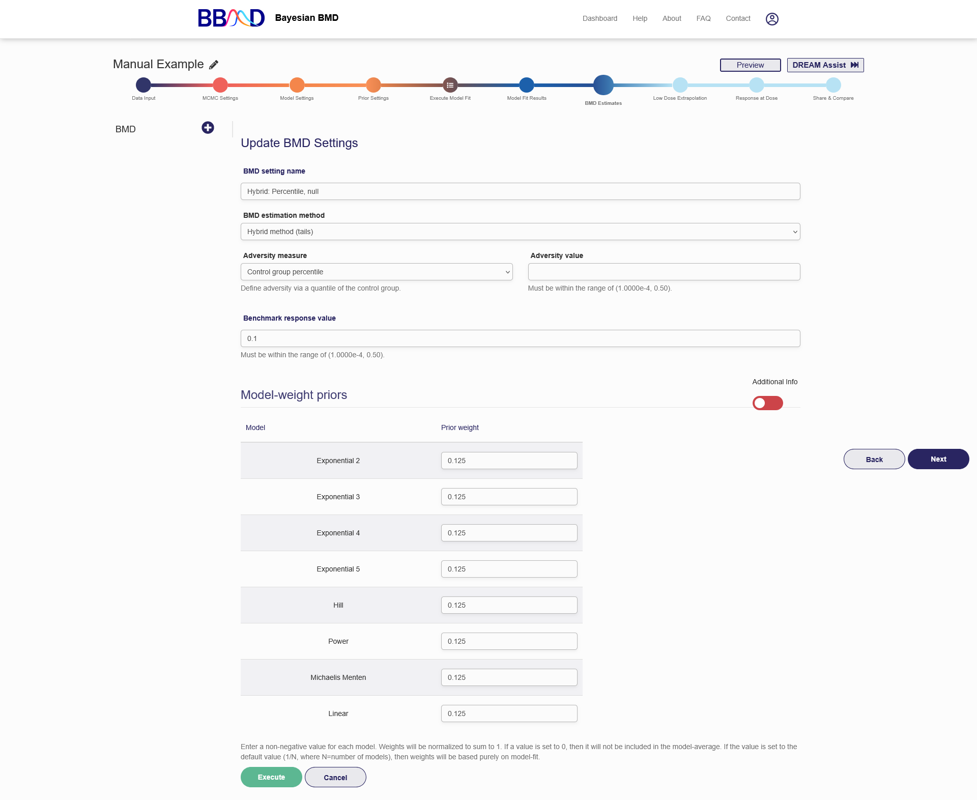
Figure 2.14. Settings for Continuous Data BMD Calculation Based on Tails

 

Once the BMD analysis is successfully created, the name of the analysis will show on the left panel and the results will be displayed on the right panel (shown previously in Figure 2.11). To add a new BMD analysis, click the plus button in the left column and repeat steps (1) to (6) above. To edit or delete an existing BMD analysis, click the pencil in the upper right corner. From here you can change the name, estimation method, adversity measure, adversity value, BMR value, or model weights the same way as when the analysis was created. To save the changes made, click “Execute” on the bottom of the page. To delete this analysis, click “Delete”. To cancel the modification, click ‘Cancel’.

For both types of estimation methods, an adversity measure needs to be specified. For “Central Tendency” there are three options to specify an adversity:

1. Relative change:

For this option, you need to input a value of relative change, e.g., 20%. This means that if the central tendency changes 20% from the control, it will be considered as adverse and the BMD will be calculated accordingly, using the following equation:

𝑓(𝐵𝑀𝐷) ± 𝑓(0) = 𝑅𝑒𝑙𝑎𝑡𝑖𝑣𝑒 𝐶ℎ𝑎𝑛𝑔𝑒 × 𝑓(0)

where 𝑓(∙) represents a continuous dose–response model fit to the central tendency of the data (i.e., the median under the lognormality assumption). The BMD stands for the dose level that satisfies the selected definition equation. The plus/minus sign on the left-hand side is related to the dose-response trend, if increasing, then it is “+”, otherwise it is “-”.

2. Absolute change:

For this option, you need to input a value of absolute change, e.g., 3.2. This means that if the central tendency changes 3.2 from the control, it will be considered as adverse and the BMD will be calculated accordingly, using the following equation:

𝑓(0) ± 𝐴𝑏𝑠𝑜𝑙𝑢𝑡𝑒 𝐶ℎ𝑎𝑛𝑔𝑒 = 𝑓(𝐵𝑀𝐷)

The plus/minus sign on the left-hand side is related to the dose-response trend, if increasing, then it is “+”, otherwise it is “-”.

3. Cutoff:

For this option, you need to input a value of cutoff, e.g., 22.5. This means that if the central tendency is equal to the cutoff value specified, it will be considered as adverse and the BMD will be calculated accordingly, using the following equation:

𝑓(𝐵𝑀𝐷) = 𝑐𝑢𝑡𝑜𝑓𝑓

The allowable range for the values of these three options will be automatically calculated based on the trend of the dose-response data and shown.

For the “Hybrid Method (tails)” estimation method, an adversity value must be specified in addition to a BMR value. The hybrid approach considers any response above or below (i.e., corresponding to increasing or decreasing trend) the adversity value as abnormal; thus, the BMD is the dose level where the proportion of the abnormality has increased a certain percent (i.e., BMR) compared with the control. There are two options to specify an adversity:

1. Absolute cutoff value:

For this option, you need to input a value of a cutoff. Then, depending on increasing or decreasing dose-response trend, above or below this value will be considered as adverse.

2. Control group percentile:

For this option, you need to input a percentile value of the control. Then, the below 1st percentile or above 99th percentile of the control distribution is considered as adverse depending on decreasing or increasing.

Mathematically, for increasing trend, the hybrid BMD definition can be expressed as 

𝑄(0) − 𝑄(𝐵𝑀𝐷) = 𝐵𝑀𝑅 for added risk,

((0)−𝑄(𝐵𝑀𝐷))/(1−𝑄(0)) = 𝐵𝑀𝑅 for extra risk;

For decreasing trend,

𝑄(𝐵𝑀𝐷) − 𝑄(0) = 𝐵𝑀𝑅 for added risk,

((𝐵𝑀𝐷)−𝑄(0))/𝑄(0) = 𝐵𝑀𝑅 for extra risk;

where 𝑄(0) represents the quantile of the adversity value at control dose and 𝑄(𝐵𝑀𝐷) represents the quantile of the adversity value at the BMD level

Categorical Data

Figure 2.15 is a screenshot of the “BMD estimates” tab for a categorical dataset. To create a BMD analysis, you need to follow the five steps below:

1. Name the BMD analysis using an easily identifiable name in the “Model name” box.
2. Specify a BMR value in the “Benchmark response value” box.
3. Select a severity level from the “Severity Level” drop-down list. The number of options equals to levels of the input dataset.  
4. Give prior model weight to the models included in this analysis. Similarly, “Additional Info” section provides you further info on the performances of each model fitting. The prior weight, PPP value and the calculated weights for each model are provided when you change the slider in the right side of the page below “Additional Info” to green. The prior weight will influence the estimation of model averaged BMD value. Giving 0 weight to a particular model can exclude the model from model-averaged BMD calculation. The sum of the weights assigned to the individual models are not necessarily required to be 1. The system will automatically convert them. For example, if you give 1 to Logistic model and 3 to Cloglog model, the system will convert these values to 25% prior weight for the Logistic model and 75% prior weight for the Cloglog model.
5. Click the “Execute” button to execute the BMD analysis using the settings just specified.

Once the BMD analysis is successfully created, the name of the analysis will show on the left panel and the results will be displayed on the right panel (previously shown in Figure 2.11). To add a new BMD analysis, click the plus button in the left column and repeat steps (1) to (5) above. To edit or delete an existing BMD analysis, click the pencil in the upper right corner. From here you can change the name, BMR value, severity level, or model weights the same way as when the analysis was created. To save the changes made, click “Execute” on the bottom of the page. To delete this analysis, click “Delete”. To cancel the modification, click “Cancel”.

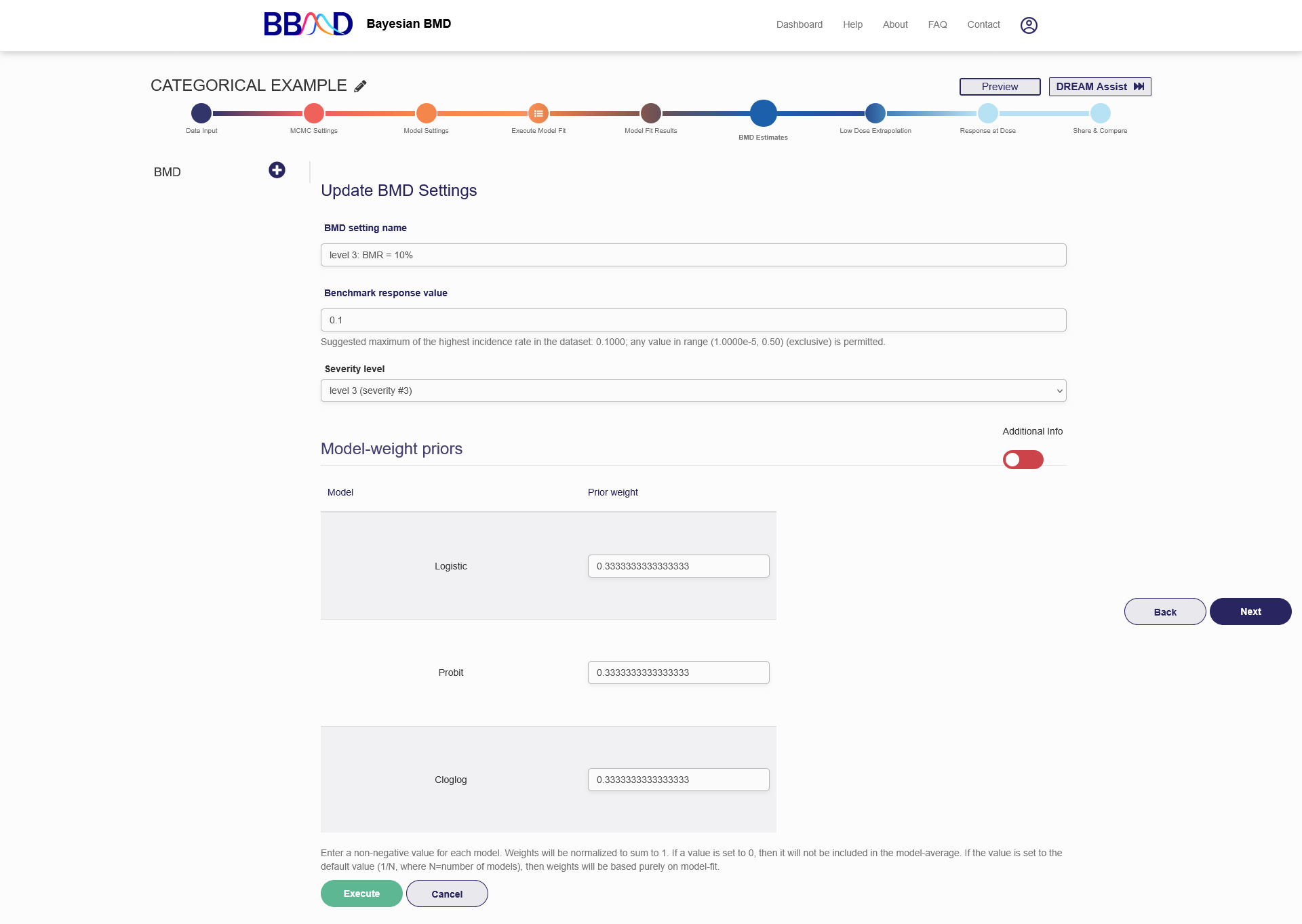
Figure 2.15. Settings for a Categorical Data BMD

The BMD is defined based on “Central Tendency” for each severity level. The BMD are calculated for both the added risk and extra risk at each severity level. For the two risks, the BMDs are defined by the following equations, respectively:

Added risk: 𝑓(𝐵𝑀𝐷) − 𝑓(0) = 𝐵𝑀𝑅, Extra risk: (𝑓(𝐵𝑀𝐷)−𝑓(0))/(1−𝑓(0)) = 𝐵𝑀𝑅;

where 𝑓(∙) represents a dichotomous dose–response model. BMR stands for benchmark response, which is a specified increase in the probability of response and is commonly set at 10%, 5%, or 1%.

Before calculating a model averaged BMD, a posterior sample of the BMD from each individual model should be obtained. The process to get the posterior sample was described in the previous three sections. Here, we focus on the method to get model averaged BMD.

In this step, the prior model weight specified by users will be used in the posterior model weight calculation. The function is shown below. The 𝑚̂ for each model is calculated using the same procedure described in the previous section.

Pr(ℳ_𝑗|𝐷𝑎𝑡𝑎) = 𝑚̂_𝑗 Pr(ℳ_𝑗)/(∑ 𝑚̂ _𝑡Pr(ℳ𝑡))

Based on the function above, we know that the posterior weight of a model will be 0 if the prior weight for the model is specified as 0. That is, the model with 0 weight will be excluded from the analysis.

For each model, we have posterior sample of BMD with the same length as the model parameters. Using default value, we should have:

𝐵𝑀𝐷1−1, 𝐵𝑀𝐷1−2, … , 𝐵𝑀𝐷1−15000 for model 1
𝐵𝑀𝐷2−1, 𝐵𝑀𝐷2−2, … , 𝐵𝑀𝐷2−15000 for model 2

Then the posterior sample of model averaged BMD is calculated as a mixture distribution over all models:

Pr(𝐵𝑀𝐷_𝑚𝑎|𝐷𝑎𝑡𝑎) = ∑ Pr (𝐵𝑀𝐷_𝑗 |𝑀_𝑗 , 𝐷𝑎𝑡𝑎)Pr (𝑀_𝑗 |𝐷𝑎𝑡𝑎)

That is:

𝐵𝑀𝐷_{𝑀𝐴−15000} = 𝐵𝑀𝐷_1−15000 × 𝑤₁ + 𝐵𝑀𝐷_2−15000 × 𝑤₂ + ⋯

Therefore, we will have the same size of posterior sample for model averaged BMD. 𝑤₁, 𝑤₂, … are posterior model weight (prior model has been integrated) calculated in the previous section.

G. Probabilistic RfD Estimation

On this page, you can calculate the RfD estimates of your interest using your previously calculated BMD estimates. The RfD estimate settings are the same for each data type.

 

Figure 2.16 is a screenshot of the “RfD estimates” tab. To create a RfD analysis, you need to follow the eleven steps below:

1. Name the RfD analysis in the “RfD analysis name” box
2. Specify the dose units in the “Dose Units” box

(Optional) Choose a random seed for the “Random number seed” box

3. Select a BMD analysis to be used as the point of departure. Your BMD analyses from the previous tab will be the possible selections in the drop-down menu.

Specify the Allometric Scaling settings. Select a test species from the “Test species” drop-down menu. Specify the test species body weight in the “Test species body weight” box. Choose a human body weight in the “Human body weight” box. Lastly, specify the Allometric scaling exponent mean and standard deviation in the two corresponding boxes. For each species you choose the default values for the parameters in “Allometric Scaling” section will automatically be displayed.

4. Give an Animal to Human Uncertainty geometric mean and geometric standard deviation. These two values go in their respective boxes.
5. Specify Duration of Exposure details to extrapolate non-chronic exposures to chronic exposures. Select the duration of exposure from the drop-down menu. Then give the short-term exposure geometric mean and geometric standard deviation in the corresponding boxes.
6. (Optional) Add up to two additional uncertainties. Each additional uncertainty requires a name, geometric mean, and geometric standard deviation. These choices go in the respective boxes.
7. Specify the Human Variability geometric mean and geometric standard deviation in the corresponding boxes.
8. Give the target population-based incidence in the I* box.
9. Click the “Save” button to execute the RfD analysis using the settings just specified.

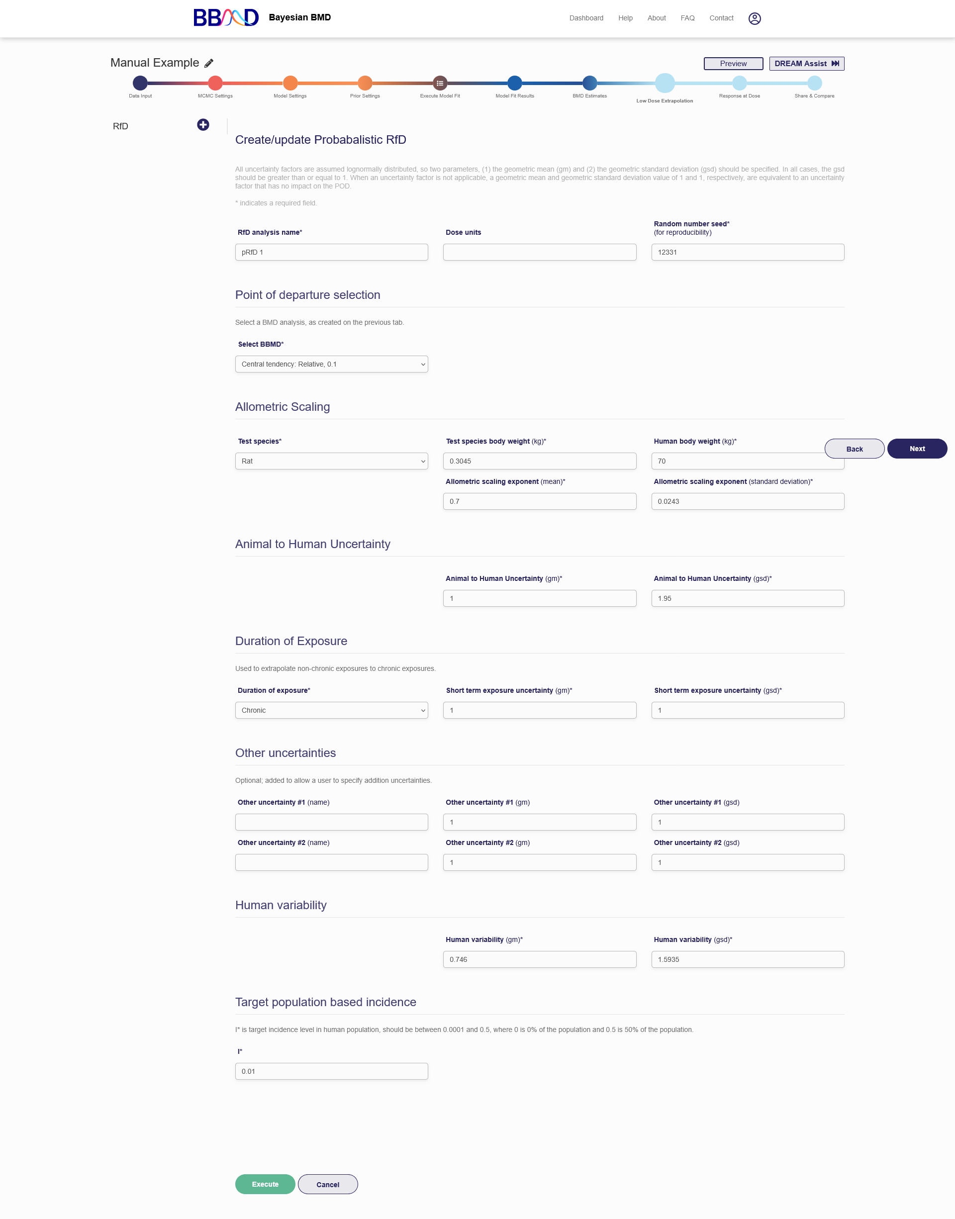
Figure 2.16. Beginning of the RfD analysis tab

 

Once the RfD analysis is successfully created, the name of the analysis will show on the left panel and the results will be shown on the right panel as shown in Figure 2.17. To add a new RfD analysis, click the plus button in the left column and repeat steps (1) to (11) above. To edit or delete an existing RfD analysis, click the pencil in the upper right corner. From here you can change all analysis settings the same way as when the analysis was created. To save the changes made, click “Update” on the bottom of the page. To delete this analysis, click “Delete”.

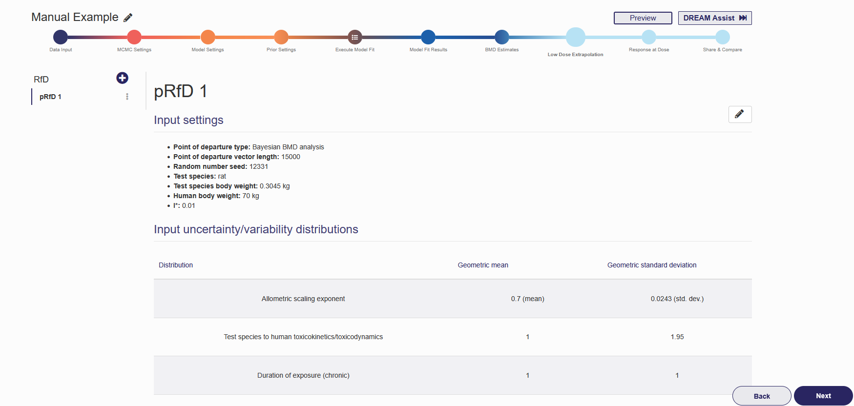
Figure 2.17. RfD Estimate results shown after RfD analysis finishes

H. Risk/Response at Dose

On this page, you can calculate the RAD (Response at Dose) estimates of your interest. The settings for RAD analyses using dichotomous data and continuous data are identical. The only difference from these two data types and categorical data is that a specified severity level is required for categorical data.

Figure 2.18 is a screenshot of the "Risk at Dose” tab (This tab is called “Response at Dose” for continuous and categorical data). To create a new RAD analysis, you need to follow the five steps below:

1. Name the RAD analysis using an identifiable name in the “Model Name” box.
2. Specify a dose value in the “Dose value” box.
3. Only for categorical data – Choose a severity level from the “Severity level” drop-down menu.
4. Give prior model weights to the models included in this analysis. Giving 0 weight to a particular model can exclude the model from model-averaged RAD calculation. The sum of the weights assigned to the individual models are not necessarily required to be 1. The system will automatically convert them.
5. Click the “Save” button to execute the RAD analysis using the settings just specified.

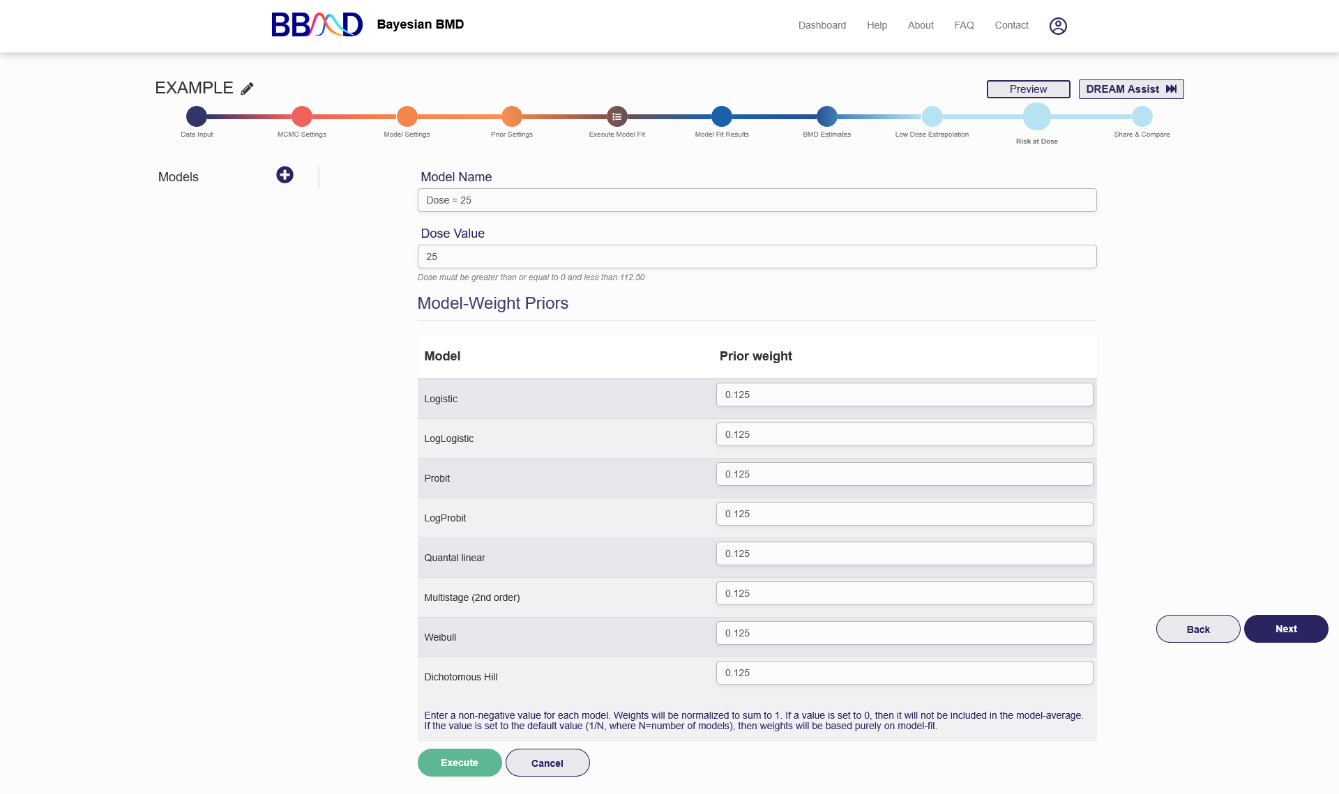
Figure 2.18. Risk at Dose analysis for Dichotomous Data

Once the RAD analysis is successfully created, the name of the analysis will be shown on the left panel and the results will be shown on the right as seen in Figure 2.19. To add a new RAD analysis, click the plus button in the left column and repeat steps (1) to (5) above. To edit or delete an existing RAD analysis, click the pencil in the upper right corner. From here you can change all analysis settings the same way as when the analysis was created. To save the changes made, press “Update” on the bottom of the page. To delete this analysis, press “Delete”.

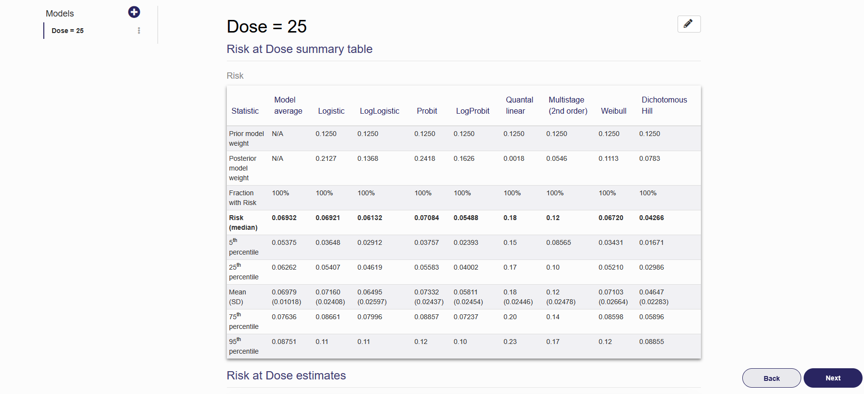
Figure 2.19. RAD Estimate results shown in on the “Risk at Dose” tab

I. Share the Analysis

The final tab for this analysis is the “Share” tab, shown in Figure 2.20. By default, all analyses in a personal account can only be accessed by the owner of the account. If you would like to share your analysis with others, you can change the settings from “Private” to “Send Back”, “Share”, “Send to a Peer”, or “Dream Assist”. The public setting (i.e., “Share”) allows you to send the created URL to others for them to access and review (but not edit) the analysis. 

You can also export the results of the analysis into Word or Excel formats. Before exporting results, you can customize the parts of the analysis included on the reports. By clicking “show more” on the right side of the page, the customization options will appear. Here you can specify the BMD results, RAD results, or model summaries to be included. If you wish to change the report settings in the future, you can return to this analysis and export a new report. Exporting the results will send a link to your account’s email where you can download the reports. 

At any time during the updating or reviewing stage, if you want to change to another existing analysis, you can click the “Dashboard” button on the top right corner to switch to the summary page for the existing analyses and access another analysis

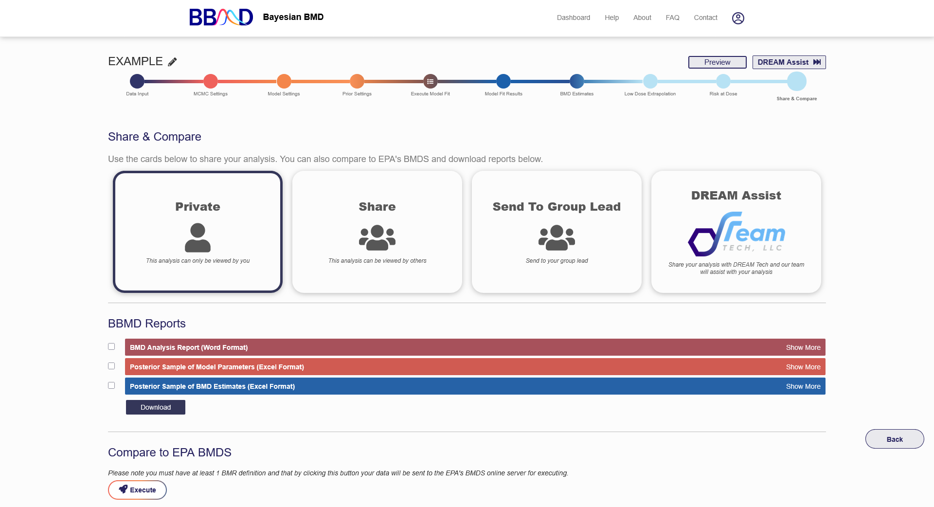
Figure 2.20. “Share” tab for a BMD analysis using a single dataset